Understanding the Nature of Oil Fluctuations
Using 1 Neutral Network Moving Average: A
Study on the Returns of Crude Oil Futures
Jacinta Chan Phooi M’ng
University of Malaya Kuala Lumpur
Malaysia 03 7967 3833
Rozaimah Zainudin
University of Malaya Kuala Lumpur
Malaysia 03 7967 3904 [email protected]
Azmin Azliza Aziz
University of Malaya Kuala Lumpur
Malaysia 03 7967 3836 [email protected]
ABSTRACT
This paper describes the profitability of technical trading rules which are enhanced by the use of neural networks on crude oil futures contracts traded on Chicago Merchantile Exchange and on Bursa Derivative Malaysia. The profitable returns on the futures contract on crude light oil futures traded from 2/1/2008 to 31/12/2014 offer a piece of evidence on the ability of technical trading rules using neural networks to outperform the threshold benchmark, buy and hold. The results here suggest that it is worthwhile to design, build and develop more robust, machine learning algorithms like neural networks enhanced moving average technical indicator to enhance portfolio returns. The conclusion drawn is that neural network can be used in technical analysis as a predictor for futures market prices.
Keywords
1. INTRODUCTION
The collapse of more than 50% in global crude oil price since middle of 2014 strengthened the US dollar against other currencies, leading to chaotic financial markets and throwing hurdles in US oil exports. Therefore, understanding the nature of the stochastic behavior of oil fluctuations is of crucial importance for decision and policy makers not only in the financial markets and at national level economies (Nazlioglu et al. 2013, Cevik and Sedik, 2011). Thus, academic studies to explain the trend in prevailing prices are in the order of the day (Cashin and Pattillo, 2000, Cashin and McDermott, 2001). The oil crisis has become a controversial issue as the oil prices record extreme movements with this high volatility attributing largely to the high demand in midst of low and unstable supply due to geopolitical conflict (Kilian, 2009). Excessive speculation activities in the commodity and futures markets also contributed to this high volatility (Singleton, 2012).
In view of these factors, this study arises to propose an innovated technical indicator using neural network to investigate the behavior of crude light oil futures FCLO) prices traded in the world’s largest exchange, Chicago Mercantile Exchange (CME) in an attempt to decipher trends in this and other oil commodity futures prices like soybean oil futures (FSO) traded on CME and crude palm oil futures (FCPO) traded on CME and Bursa Derivatives Malaysia (BDM).
More than 60% of commodity trading advisors and 40% of foreign exchange currency traders use technical analysis in making investment decisions at trading firms and investment banks (Allen and Taylor, 1990). Professional traders in the model trading desk in these large institutions are trading according to some proprietary trading models which are not readily available in the market. Algorithm technical trading of the professional model trading desk of large financial institutions encompasses quantitative methods according to appropriate algorithms to generate automated trading decisions. This research explores some of the quantitative methods behind some of these algorithm trading models. Kaufman (1998) writes that quantitative methods for evaluating price movements and making trading decision have become a dominant part of market analysis. Quantitative traders and analysts are in huge and urgent demand in most mature financial markets. Interest in high frequency trading and online trading algorithm has grown markedly over recent years (Masteika, Rutkauskas 2012, Neely et al. 2009). Accompanying this interest is the number of studies in computational trading algorithms that users find useful for investment timing (Lukac et al., 1988; Brock et al.,1992; Irwin, Park, 2009, Levich and Thomas, 1993, Gencay, 1998, Frenandez et al., 2012).
moving average rules could capture information ignored by their linear counterparts (Lee, Mather, 2004). Brock et al.(1992) finds that the most popular moving average rule is the 1-200 rule, of which the short period is one day and the long period is 200 days while other common standards include the 1-50, 1-150, 5-200, and 2-200 rules. Nevertheless, many have also highlighted the existence for this kind of profitability tends to diminish over time especially so for the last decade (Olson, 2004). To outperform the financial markets, increasingly complicated trading rules are needed (Lee, Mathur, 1995, Olsen, 2004), which might be a consequence of efficient market conditions in these markets (Fama, 1965, Black, 1971). If that were true, logically it follows that no profitable position can be gained from trading rule since the prices of these markets would have already reflected all relevant information.
Studies have shown the existence of time-varying volatility in financial and economic time-series data (Andrada-Felix and Fernandex-Rodriquez, 2008). Many have suggested that the volatility of time series is non-monotone (Bollerslev,1990) and that time-varying volatility has influenced optimal portfolio configurations (Pukthuanthong-Le et al., 2006). Despite this time-varying volatility element, most technical analyses have deployed simple moving average techniques in their estimations. In the light of this criticism (Olson, 2004) that technical trading techniques are still lacking in accounting for varying volatility clustering found in most financial time-series data, this research introduces a neural network enhanced moving average to decipher the varying trends in the market. The main rationale behind the introduction of using neural network to apportion weights through machine learning between the moving average and the actual closing price is enhance the possible abnormal returns in these futures contracts.
Financial price time series prediction has recently garnered significant interest among investors and professional analysts (Zhang, 2012). Historically, in academic studies (Fama, 1965) stock prices were seen as a random time sequence with noise, however, in the real financial markets, the fluctuation behaviors of the markets are not invariant (Zhang, 2012). Recent studies show a number of analysis methods have utilized artificial neural networks to predict stock price trends (Gencay, Stengos, 1998, Fernandez, 2013). The backpropagation neural network is a neural network training algorithm for financial forecasting (Yao et al., 1999). Multilayer neurons is one of the popular neural networks as it has the capability of complex mapping between inputs and outputs that makes it possible to approximate nonlinear function. In this present work, 10 multilayer neurons backpropagation network with 2 periods delay is applied.
[1]
Extending the research of Yao et al. (1999) using neural network to combine different technical trading indicators like Brock et al (1992) moving averages (MA), this study investigates the viability of this method fast forward to current period. Different from Yao et al. (1999), this study employs a third method using 20 days moving average, to generate adaptive abnormal returns. This is in accordance with recent findings that statistical learning methods have produced better out-of-sample results than most of the single and fixed moving average rules (Andrada-Felix and Fernandez-Rodriquez, 2008).
This paper evaluates the efficacy of technical trading rule like simple moving average, against neural network of closing prices and the neural network using closing prices and moving averages as inputs. The passive buy-and-hold strategy serves as the control. The significance of this research is in the finding of market anomalies, the hypothesis of excess returns above the threshold buy-and-hold in the long run holds true.
This paper’s objectives are twofold: the study first investigates the volatility clustering patterns of Chicago Merchant Exchange Crude Light Oil Futures (CLO) from 2004 to 2013; and then it proposes an innovated Neural Network enhanced Moving Average (NNeMA) to decipher the trends in FCLO, Soybean Oil Futures (FSO) traded in CME and Crude Palm Oil Futures (FCPO) traded in CME and BDM. The innovated neural network enhanced moving average 20, NNeMA adjusts automatically to the prevailing market condition by first recognizing the prevailing volatility and thus market state that the market is in, and then adjusts its parameter accordingly.
This paper is structured as follows. In the next section, a brief data analysis of FCLO, FSO and FCPO is presented. Section 3 discusses the trading technique methods, concentrating on neural network of 20 days moving average and closes. Section 4 discusses the empirical results and finding, while Section 5 concludes.
2. DATA ANALYSIS
The purpose of this section is to examine the volatility of the returns of these oil futures. The daily closing prices for CME’s Crude Light Oil Futures (FCLO), CME’s Soybean Oil Futures (FSO) and Bursa Derivatives Malaysia’s Crude Palm Oil Futures (FCPO) for the period January 2, 2004 to December 31, 2013 are used for this purpose. The prices are collected from Bloomberg. These prices are transformed into returns series using the natural log procedure in the return equation below:
100 ) /
ln(p p 1 x
where rt represents returns of FCLO, FSO and FCPO at period t, pt represents the series’ closing price at period t and pt-1 denotes the closing price at period t-1.
The results, presented in Table 1, show that the average return for all three tested series are between 0.03% to 0.04%. The skewness, kurtosis (from 5 to 7) and Jarque-Bera test results further validate that these series are non-normally distributed and display leptokurtic characteristics.
FCLO FSO FCPO
Mean 0.04% 0.04% 0.03%
Median 0.11% 0.00% 0.00%
Maximum 8.93% 7.84% 9.69%
Minimum -10.05% -7.04% -10.90%
Std. Dev. 2.04% 0.02% 0.02%
Skewness -0.27 0.06 -0.21
Kurtosis 5.14 4.99 7.17
Jarque-Bera 509.88 463.06 2049.33
Probability 0.0000 0.000 0.000
Table 1: Statistical Properties of the FCLO, FSO and FCPO
The data analysis ascertains that volatilities in these oils are in clusters and thus our estimation models should therefore be dynamic in nature. These observations infer that these oil futures prices display dynamic variance characteristics. The presence of dynamically changing variance validates our research decision to use neural network to apportion different weights to the inputs, daily closes and its 20 day moving average.
The estimation techniques are those used in Brock et al. (1992), Lukac et al. (1988), Gencay, Stengos (1998) and Yao et al. (1999). The study tests if one or more of the technical trading rules are superior to the passive buy-and-hold strategy which is commonly used as benchmark (Fama, 1965). Using a combination of current close and 20 days moving average for a multilayer neural network, this study adopts a similar testing approach based on technical trading rules specified by Yao et al. (1999). The following section summarize the techniques used in the analysis, including that of the benchmark model, buy and hold.
3. TRADING METHODS
general, the technical trading rules generates higher returns than the passive buy-and-hold strategy and in particular, the Neural Network enhanced Moving Average (NNeMA) outperforms the most optimized moving average commonly used by Brock et al. (1996), Lukac et al. (1998) and the market practitioners and the neural network of closing prices. The approach is to i) backtest and find the most optimized moving averages for these three series, ii) use the closing prices of these series on simple back propagation ANN model to generate a series of forecast values, which are then compared to the actual closing prices to determine the trading signal, and iii) use the 20 days moving averages and the closing prices as inputs to the ANN model. The training period is from January 2, 2004 to December 31, 2011, while the validation period is from January 2, 2012 to December 31, 2012 and the out-of-sample period is from January 2, 2013 to December 31, 2013.
A trading model should meet the following criteria: i) it should not produce huge losses or exhibit any net large losses in any of the years; ii) the model should work well both in testing stage and in practice, and that it should adjust automatically to shifts in parameter; and iii) it must produce abnormal returns even after accounting for transaction and slippage costs.
The following notes summarize the techniques used in the analysis, including that of the benchmark model.
3.1 Passive Buy and Hold Strategy
The benchmark for any model is that the returns must surpass of the passive strategy of buy and hold (Fama, 1965). The excess return is termed as abnormal return. If the strategy can outperform the benchmark buy-and-hold for different periods of time, then the market prices are not random (Fama, 1965).
3.2 Optimal Day Simple Moving Averages (SMA) Trading Rule
whereSMA is the simple moving average,
n is 20-day moving-average length, and
Ct is the closing price at period t.
Trading Strategy:
If Ct >SMAnt,
then buy else sell.
3.3 ANN Model using Closing Prices only
The second method is to use the closing prices as input into a simple back propagation neural network model to produce predicted price for the next period as output. The error backpropagation neural network, a recursive gradient descent method that minimises the sum of squared errors of the system by moving down the gradient error curve. is used because multilayer perceptron is one of the most prevalent neural networks that has the capability to map between inputs and outputs. This makes it possible to approximate nonlinear function. The values of the weights are determined by an iterative learning process and their transformation at each successive layer is determined by a specific transfer function. As for the transformation functions, F is a logarithmic function and G is a hyperbolic tangent function.
[1]
In this simulation, first the closing prices are fed into a 10 layers, 2 periods delay configuration neural network model using January 2, 2004 to December 31, 2011 as the training period. The trained neural network model that has the least normalized mean square error (NMSE) between the outputs and the actual closes in the out-of-sample period is selected for use to predict future direction. According to Yao et al., 1999, a prediction that follows closely the trend of the actual target would result in a low NMSE. Lastly, the resulting outputs are used in the trading method to determine the trading signal by comparing the predicted output for the next period with the actual current close. If the predicted output for the next day is higher than the current close, the signal will be processed as a buy long. The objective of this exercise is to determine if the abnormal returns arising from utilizing the knowledge of tomorrow’s predicted price are significantly higher than the passive buy-and-hold control.
If ĉ t+1 > C t, then buy else sell.
where,
ĉ t+1is the predicted close output for the next period, and C t is the current close.
3.4 ANN Model using Closing Prices and 20 Day moving average
The third method is to use the closing prices and 20 day moving averages as inputs into the same error back propagation neural network model, using recursive gradient descent to minimizes the sum of square errors to produce predicted price for the next period as output. A technically enhanced neural network moving average (NNeMA) developed for financial time series prediction is presented in this present work.
In this simulation, the closing prices and their 20 days moving averages are fed into the 10 layers, 2 periods delay configuration neural network model using January 2, 2004 to December 31, 2011 as the training period. The trained neural network model that has the least NMSE between the outputs and the actual closes in the out-of-sample period is selected for use to predict future direction. Finally, the resulting outputs are used in the trading method to determine the trading signal by comparing the predicted output for the next period with the actual current close. If the predicted output for the next day is higher than the current close, the signal will be buy long. The objective of this exercise is to determine if the abnormal returns arising from utilizing the knowledge of tomorrow’s predicted price are significantly higher than the passive buy-and-hold control.
Trading Strategy: If ĉ t+1 > C t, then buy else sell.
where,
ĉ t+1is the predicted close output for the next period, and C t is the current close.
4. EMPIRICAL FINDINGS
In this section, performances of the 3 trading models, are evaluated against that of the passive buy-and-hold control strategy.
above those of the other trading systems. The results show that the objectives of this research which are to find abnormal returns of the three trading systems above that of passive buy-and-hold (BH) (after taking into consideration transaction costs); and to show how the new NNeMA20 model outperforms most of the other tested trading systems, have been achieved.
It is noted in studies (Irwin and Park, 2008) and in real life trading that transaction costs account for a chunk of the trading losses and thus, it would unrealistic if transaction costs are not included in this study. The transaction costs are converted into the nearest index point(s) to account for brokerage commission including exchange and clearing fees as well as slippage. Therefore, the transaction costs for two ways for FCLO are USD4.601 (0.005 of USD0.01x10 contract size), for FSO are USD5.602 (about 0.01 of 0.0001x6) and for FCPO are RM502 (2 times of its minimum tick of RM25).
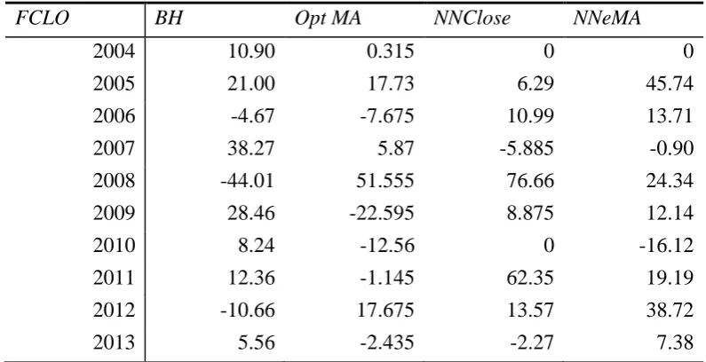
Taking transaction costs of 0.005 for each FCLO transaction, 0.01 for FSO and 2 for FCPO into consideration, the mean returns (in average percentage per year) are produced in Table 2, 3 and 4 respectively after deducting for the number of transactions generated by the trading systems. Even after taking into account the hefty transaction costs, the trading results do not differ much from the original results.
FCLO BH Opt MA NNClose NNeMA
2004 10.90 0.315 0 0
2005 21.00 17.73 6.29 45.74
2006 -4.67 -7.675 10.99 13.71
2007 38.27 5.87 -5.885 -0.90
2008 -44.01 51.555 76.66 24.34
2009 28.46 -22.595 8.875 12.14
2010 8.24 -12.56 0 -16.12
2011 12.36 -1.145 62.35 19.19
2012 -10.66 17.675 13.57 38.72
[image:9.595.105.503.355.559.2]2013 5.56 -2.435 -2.27 7.38
Table 2: Test Results on FCLO after transaction costs from 2/1/2004 to 31/12/2013
FSO BH Opt MA NNClose NNeMA
1 The commission per contract per one way at Interactive Brokers for FCLO and FSO is USD0.85 while the exchange
and regulatory fees in NYMEX where FCLO is traded are USD1.45 and in CBOT where FSO is traded are USD1.95.
2
2004 -6.74 -2.62 -31.09 -5.71
2005 1.12 -4.29 3.75 -6.85
2006 8.00 2.18 2.60 6.57
2007 19.97 4.81 -0.40 5.15
2008 -16.16 20.95 27.18 52.45
2009 7.21 5.67 11.20 -11.85
2010 17.58 1.65 7.12 1.65
2011 -5.96 -11.62 9.42 24.29
2012 -2.60 -3.70 -5.09 -4.30
[image:10.595.93.491.56.242.2]2013 -11.37 -1.72 4.02 1.60
Table 3: Test Results on FSO after transaction costs from 2/1/2004 to 31/12/2013
FCPO BH Opt MA NNClose NNeMA
2004 -379 265 8 314
2005 28 2 0 -69
2006 580 525 5 -544
2007 1055 393 623 1601
2008 -1355 409 -541 1189
2009 968 1176 1738 1790
2010 1125 658 -446 146
2011 -613 194 102 683
2012 -737 1196 443 1108
[image:10.595.94.489.307.510.2]2013 29 747 427 747
Table 4: Test Results on FCPO after transaction costs from 2/1/2004 to 31/12/2013
In summary, even after taking into consideration the hefty transaction costs, the returns for NNclose and NNeMA for FCLO, FCO and FCPO are much larger than the passive buy-and-hold control strategy as shown in Table 5.
BH Opt MA NNClose NNeMA
FCLO 67.10 46.735 170.56 144.20
FSO 10.82 11.31 28.71 63.00
Table 5: Summary of Test Results on FCLO, FSO and FCPO after transaction costs from 2/1/2004 to 31/12/2013
Similar findings by Lukac et al. (1988)[9], Brock et al. (1992)[3] and Irwin and Park (2009) [7] support the results. To compare the three models, the sum of the net % returns over the 10 years using base prices as at 2/1/2004, for FCLO, 33.00, FSO, $27.76 and FCPO, 1766.
BH Opt MA NNClose NNeMA
FCLO 198.24% 141.62% 516.86% 436.95%
FSO 40.96% 40.74% 103.42% 226.95%
FCPO 50.57% 315.12% 133.58% 394.39%
Total 288.66% 497.48% 753.86% 1,058.29%
Table 6: Net Percentage Returns for FCPO, FSO and FCPO after transaction costs from 2/1/2004 to 31/12/2013
[image:11.595.122.487.469.677.2]The moving averages, neural network close outputs and neural network enhanced moving average outputs are moving in tandem with each other for all the three series as these are all lagging technical indicators. From the observation of this study, it can be seen that these are powerful predictive indicators of future performances of these contracts as they all generate significantly higher returns than the passive control strategy of buy and hold for all these futures. Figure 1 shows the NNeMA20 and FCLO prices over the last ten years, while Figure 2 and 3 show the relationships between NNeMA20 and FSO and FCPO respectively.
Fig 2: FSO Daily Closes, MA20, NNClose and NNeMA20 for 2/1/2004 to 31/12/2013
Fig 3: FCPO Daily Closes, MA20, NNClose and NNeMA20 for 2/1/2004 to 31/12/2013
This indicates that NNeMA20 is a robust trading model and can be used for all these markets. NNeMA20 can be taken into consideration as a viable trading model for the professional model trading desk of financial institutions.
[image:12.595.111.471.296.508.2]outperforming its nearest rival, NNClose of 46% by a relatively large margin of 97%. This is consistent with the findings by Olson, 2004 that the excessive returns of yesteryears from conventional technical trading rules like moving average tend to diminish over time and new adjustable trading systems are required.
5. CONCLUSION
In the past, stock prices had been seen as random walk time sequence with noise and efforts to decipher trends with fundamental and technical analysis were rendered useless (Fama, 1965). Financial market dynamics forecasting is a focus of economic and finance research (Zhang, 2012). Artificial neural networks have good self-learning ability and have been widely used in the financial fields such as stock prices profit prediction (Zhang, 2012).
From the statistical data descriptive, these oils’ returns seem to follow similar properties to financial returns; that is, they are non-normal, with excess kurtosis and skewness.
For the period 2004 to 2013 as a sample, this study assess the efficacy of three technical trading rules; the 20 days simple moving-averages, ANN of closing prices and an ANN of closing prices and 20 days simple moving averages as inputs. The results show that all the trading models are able to outperform the passive buy-and-hold strategy. This is consistent with the studies conducted by Lukac et al.(1988), Brock et al.(1992), and Andrada-Felix
et al.(2008).
While simple moving-average rules have outdone the other technical models ex-post, ex-ante it is extremely difficult to estimate accurately the optimal lengths to be deployed (Gandolfi et al. (2008)). This research introduces a new algorithm trading system (NNeMA20) to high frequency traders in model trading desks worldwide. We compare NNeMA20 along with the other 3 technical trading models (MA and ANN of Closing Prices) with the passive buy-and-hold strategy. NNeMA20 has the ability to adjust quickly so that it can be robust in different markets and across different time frames. NNeMA20 is designed to address some of the common problems encountered by most trend trading systems like being triggered by floods of orders generated by common trading systems (like simple moving averages), being whipsawed in range market and the inability to capture the trend by entering the trend too late and exiting the trend too early.
The results show that all the algorithm trading systems generate more profits than the threshold buy-and-hold strategy, all the algorithm trading systems generate net profits in the long run and NNeMA20 generates more net profits for than the other trading systems. It can be concluded that there are trends in oil futures which can be captured in terms of abnormal profitable returns using mechanical trading systems like NNeMA20 and NNeMA20 is a robust trading system that can be implemented from past and current empirical evidence.
NNeMA20 is new technical indicator that can contribute to the profits of the model trading desk. Its ability to adjust according to market conditions points a new research direction for incremental learning trading systems. The ability of NNeMA20 to adjust according to the prevailing market condition, points a new direction for research in incremental machine learning trading systems. New adaptive new trading indicators like NNeMA20 can be applied immediately on any professional model trading desk. With artificial intelligent algorithms, neural networks can learn the behaviour of the market, whether it is trending or ranging, and adjust the algorithms automatically according to the prevailing market condition. Despite good preliminary results, future research can explore and find better fit for these and other world commodities with use of neural network enhanced wavelets.
References
Allen, H, and Taylor, M., 1990. “Charts, noise and fundamentals in the London foreign exchange market.” Economic Journal. 100: 49-59.
Andrada-Felix, J, Fernandex-Rodriquez, F. 2008. “Improving Moving Average Trading Rules with Boosting and Statistical Learning Methods.” Journal of Forecasting, 27(5): 433-449.
Black F. 1971. “Implications of Random Walk Hypothesis for Portfolio Management.” Financial Analysts Journal, 27 (2): 16-22.
Bollerslev, T. 1990. “Modelling the Coherence in Short-Run Nominal Exchange Rates: A Multivariate Generalized ARCH Model.” The Review of Economics and Statistics, 72(3): 498-505.
Brock W, Lakonishok J, LeBaron B. 1992. “Simple Technical Trading Rules and the Stochastic Properties of Stock Returns.” Journal of Finance, 47: 1731–1764.
Cashin, P., MCDermott, C.J. The Long-Run Behavior of Commodity Prices: Small Trends and Big Variability. Working Paper 01/68. International Money Fund 2001, Washington.
Cashin, P., Pattillo, C. Terms of trade shock in Africa: Are they short-lived or long-short-lived? Working Paper 00/72. International Money Fund 2000, Washington.
Fama, E F. 1965. "Random Walks In Stock Market Prices". Financial Analysts Journal, 21 (5): 55–59
Frenandez A, Frenandez F, Sosvilla S. 2013. “Genetic Algorithm for Arbitrage with More than Three Currencies” Working Paper, 12-04, Asciacion Espanola de Economia y Finanzas Internacionales.
Gehrig T, Menkhoff L. 2006. “Extended evidence on the use of technical analysis in foreign exchange.” International Journal of Finance and Economics, 11: 327-338.
Gencay R, Stengos T. 1998. “The Predictability of Security Returns with Simple Trading Rules.” Journal of Forecasting, 17: 401-414.
Gencay R. 1998. “The Predictability of Security Returns with Simple Trading Rules.” Journal of Empirical Finance, 5: 347-359.
Irwin S, Park C. 2009. “A Reality Check on Technical Trading Rule Profits in the U.S. Futures Markets.” Journal of Futures Markets, 30: 633-659.
Kilian, L. . Not all oil price shocks are alike: Disentangling demand and supply shocks in the crude oil market. American Economic Review 2009; 99(3): 1053-1069.
Kaufman P. 1998. Trading Systems and Methods. John Wiley &Sons, Third Edition.
Lee C, Mathur I. 1996. “Trading rule profits in European currency spot cross rates.” Journal of Banking and Finance, 20: 949-962.
Levich R, Thomas L. 1993. “The Significance of Technical Trading-Rule Profits in the Foreign Exchange Market: A Bootstrap Approach.” Journal of International Money and Finance, 12: 451-474.
Lukac L, Brorsen B, Irwin S. 1988. “A Test of Futures Market Disequilibrium Using Twelve Different Technical Trading Systems.” Applied Economics, 20: 623-639.
Masteika S, Rutkauskas AV. 2012. “Research on Futures Trend Trading Strategy Based on Short Term Chart Pattern.” Journal of Business Economics and Management, 13(5): 915-930.
Nazlioglu, S., Erdem, C. and Soytas, U.. Volatility spillover between oil and agricultural commodity futures markets. Energy Economics 2013; 36: 658-665.
Nazlioglu, S.Soytas, U. . World oil prices and agricultural commodity prices: Evidence from an emerging market. Energy Economics 2011; 33: 488-496.
Nazlioglu, S., Erdem, C. and Soytas, U. Volatility spillover between oil and agricultural commodity futures markets. Energy Economics 2013; 36: 658 – 665.
Olson, D. 2004. “How Trading Rule Profits in the Currency Markets Declined Over Time?” Journal of Banking and Finance, 28: 85-105.
Pukthuanthong-Le, K., Levich, R., Thomas, L. 2006. “Do Foreign Exchange Markets Still Trend?” Journal of Portfolio Management, 34: 114-118.
Singleton, K . Investor flows and the 2008 boom/bust in oil prices. Management Science 2012; 60(2): 300-318.
Szakmary, A., Shen, Q., Sharma, S.C. 2010. “Trend-following Trading Strategies in Commodity Futures: A Re-examination.” Journal of Banking and Finance, 34(2): 409-426.
Yao, J., Chew, L.T , Poh, H. 1999. “Neural Networks for Technical Analysis: A Study on KLCI” International Journal of Theoretical and Applied Finance, 2(2): 221-241.