Hydraulic and transport parameter assessment using column infiltration experiments

www.hydrol-earth-syst-sci.net/21/2263/2017/ doi:10.5194/hess-21-2263-2017

© Author(s) 2017. CC Attribution 3.0 License.

Hydraulic and transport parameter assessment using column

infiltration experiments

Anis Younes1,2,3, Thierry Mara4, Marwan Fahs1, Olivier Grunberger2, and Philippe Ackerer1 1_{LHyGES, Université de Strasbourg/ENGEES, CNRS, 1 rue Blessig, 67084 Strasbourg, France} 2_{UMR LISAH, INRA-IRD-SupAgro, 92761 Montpellier, France}

3_{LMHE, Ecole Nationale d’Ingénieurs de Tunis, Tunis, Tunisia}

4_{Université de La Réunion, PIMENT, 15 Avenue René Cassin, BP 7151, 97715 Moufia, La Réunion, France}

Correspondence to:Philippe Ackerer ([email protected]) Received: 10 June 2016 – Discussion started: 20 June 2016

Revised: 28 March 2017 – Accepted: 6 April 2017 – Published: 3 May 2017

Abstract. The quality of statistical calibration of hydraulic and transport soil properties is studied for infiltration exper-iments in which, over a given period, tracer-contaminated water is injected into an hypothetical column filled with a homogeneous soil. The saturated hydraulic conductivity, the saturated and residual water contents, the Mualem–van Genuchten shape parameters and the longitudinal dispersiv-ity are estimated in a Bayesian framework using the Markov chain Monte Carlo (MCMC) sampler. The impact of the kind of measurement sets (water content, pressure inside the col-umn, cumulative outflow and outlet solute concentration) and that of the solute injection duration is investigated by ana-lyzing the calibrated model parameters and their confidence intervals for different scenarios. The results show that the in-jection period has a significant effect on the quality of the estimation, in particular, on the posterior uncertainty range of the parameters. All hydraulic and transport parameters of the investigated soil can be well estimated from the experi-ment using only the outlet concentration and cumulative out-flow, which are measured non-intrusively. An improvement of the identifiability of the hydraulic parameters is observed when the pressure data from measurements taken inside the column are also considered in the inversion.

1 Introduction

The soil parameters that influence water flow and contami-nant transport in unsaturated zones are not generally known a priori and have to be estimated by fitting model responses

to observed data. The unsaturated soil hydraulic parameters can be (more or less accurately) estimated from dynamic flow experiments (e.g., Hopmans et al., 2002; Vrugt et al., 2003a; Durner and Iden, 2011; Younes et al., 2013). Several authors have investigated different types of transient experiments and boundary conditions suited for a reliable estimation of soil hydraulic properties (e.g., van Dam et al., 1994; Šim˚unek and van Genuchten, 1997; Inoue et al., 1998; Durner et al., 1999). Soil hydraulic properties are often estimated using inversion of one-step (Kool et al., 1985; van Dam et al., 1992) or mul-tistep (Eching et al., 1994; van Dam et al., 1994) outflow ex-periments or controlled infiltration exex-periments (Hudson et al., 1996).

Kool et al. (1985) and Kool and Parker (1988) suggested that the transient experiments should cover a wide range of water contents to obtain a reliable estimation of the parame-ters. Van Dam et al. (1994) have shown that more reliable pa-rameter estimates are obtained by increasing the pneumatic pressure in several steps instead of a single step. The mul-tistep outflow experiments are the most popular laboratory methods (e.g., Eching and Hopmans, 1993; Eching et al., 1994; van Dam et al., 1994; Hopmans et al., 2002). How-ever, their application is limited by expensive measurement equipment (Nasta et al., 2011).

smaller estimation errors for model parameters than the se-quential inversion of hydraulic properties from the water con-tent and/or pressure head followed by the inversion of trans-port properties from concentration data (Mishra and Parker, 1989).

Inoue et al. (2000) performed infiltration experiments us-ing a soil column of 30 cm. Pressure head and solute con-centration were measured at different locations. A constant infiltration rate was applied to the soil surface and a balance was used to measure the cumulative outflow. They showed that both hydraulic and transport parameters can be assessed by the combination of flow and transport experiments.

Furthermore, infiltration experiments were often con-ducted in lysimeters for pesticide leaching studies. Indeed, lysimeter experiments are generally used to assess the leach-ing risks of pesticides usleach-ing soil columns of around 1.2 m depth which is the standard scale for these types of ex-periments (Mertens et al., 2009; Kahl et al., 2015). Be-fore performing the column leaching experiment, several infiltration–outflow experiments are often realized to esti-mate the soil hydraulic parameters (Kahl et al., 2015; Dusek et al., 2015).

The key objective of the present study is to evaluate the reliability of different experimental protocols for estimating hydraulic and transport parameters and their associated un-certainties for column experiments. We consider the flow and the transport of an inert solute injected into a hypotheti-cal column filled with a homogeneous sandy clay loam soil. We assume that flow can be modeled by the Richards’ equa-tion (RE) and that the solute transport can be simulated by the classical advection–dispersion model. Furthermore, the Mualem and van Genuchten (MvG) models (Mualem, 1976; van Genuchten, 1980) are chosen to describe the retention curve and to relate the hydraulic conductivity of the unsatu-rated soil to the water content. The estimation of the flow and transport parameters through flow–transport model inversion is investigated for two injection periods of the solute and dif-ferent data measurement scenarios.

Inverse modeling is often performed using local search al-gorithms such as the Levenberg–Marquardt algorithm (Mar-quardt, 1963). The latter is computationally efficient to evalu-ate the optimal parameter set (Gallagher and Doherty, 2007). Besides, the degree of uncertainty in the estimated param-eters, expressed by their confidence intervals, is often cal-culated using a first-order approximation of the model near its minimum (Carrera and Neuman, 1986; Kool and Parker, 1988). However, as stated by Vrugt and Bouten (2002), pa-rameter interdependence and model nonlinearity occurring in hydrologic models may violate the use of this first approx-imation to obtain accurate confidence intervals of each pa-rameter. Therefore, in this work, the estimation of hydraulic and transport parameters is performed in a Bayesian frame-work using the Markov chain Monte Carlo (MCMC) sampler (Vrugt and Bouten, 2002; Vrugt et al., 2008). Unlike classi-cal parameter optimization algorithms, the MCMC approach

generates sets of parameter values randomly sampled from the posterior joint probability distributions, which are useful to assess the quality of the estimation. The MCMC samples can be used to summarize parameter uncertainties and to per-form predictive uncertainty (Ades and Lu, 2003).

Hypothetical infiltration experiments are considered for a column of 120 cm depth, initially under hydrostatic condi-tions, free of solute and filled with a homogeneous sandy clay loam soil. Continuous flow and solute injection are per-formed during a time periodTinj at the top of the column and with a zero-pressure head at the bottom. The unknown parameters for the water flow are the hydraulic parameters: ks(L T−1), the saturated hydraulic conductivity;θs(L3L−3), the saturated water content;θr (L3L−3), the residual water content; andα(L−1) andn(−), the MvG shape parameters. The only unknown parameter of the tracer transport is the longitudinal dispersivity,aL(L).

Several scenarios corresponding to different sets of mea-surements are investigated to address the following ques-tions:

1. Can we obtain an appropriate estimation of all flow and transport parameters from tracer-infiltration exper-iments, even though a limited range of water contents is covered (only moderately dry conditions are obtained because of gravity drainage conditions prescribed at the bottom of the soil column)?

2. What is the optimal set of measurements for the esti-mation of all the parameters? Can we use only non-intrusive measurements (cumulative outflow and con-centration breakthrough curve) or are intrusive mea-surements of pressure heads and/or water contents in-side the column unavoidable?

3. Is there an optimal design for the tracer injection? For this purpose, synthetic scenarios are considered in the sequel in which data from numerical simulations are used to avoid the uncontrolled noise of experiments that could bias the conclusions.

The paper is organized as follows. The mathematical mod-els describing flow and transport in the unsaturated zone are detailed in Sect. 2. Section 3 describes the MCMC Bayesian parameter estimation procedure used in the DREAM(ZS) sampler. Section 4 presents the different investigated scenar-ios and discusses the results of the calibration in terms of mean parameter values and uncertainty ranges for each sce-nario. Conclusions are given in Sect. 5.

2 Unsaturated flow–transport model

ver-tical soil column is modeled with the one-dimensional pres-sure head form of the RE:

      

c (h)+Ss θ θS ∂h ∂t = ∂q ∂z

q=K (h)

∂h ∂z−1

, (1)

where h (L) is the pressure head; q (L T−1) is the Darcy velocity; z (L) is the depth, measured as positive in the downward direction;Ss (−) is the specific storage;θandθs (L3L−3) are the actual and saturated water contents, respec-tively;c (h)(L−1) is the specific moisture capacity; andK (h) (L T−1) is the hydraulic conductivity. The latter two parame-ters are both functions of the pressure head. In this study, the relations between the pressure head, conductivity and water content are described by the following standard models of Mualem (1976) and van Genuchten (1980):

Se(h)=

θ (h)−θr θs−θr

=

  

1

1+ |αh|nm h <0

1 h≥0

K (Se)=KsSe1/2

h

1−1−Se1/m

mi2

, (2)

where Se (−) is the effective saturation,θr (L3L−3) is the residual water content,Ks(L T−1) is the saturated hydraulic conductivity, and m=1−1/n,α (L−1) and n (−) are the MvG shape parameters.

The tracer transport is governed by the following convection–dispersion equation:

∂ (θ C)

∂t + ∂ (qC) ∂z − ∂ ∂z

θ D∂C ∂z

=0, (3)

where C (M L−3) is the concentration of the tracer, D (L2T−1) is the dispersion coefficient in whichD=alq+dm andal (L) is the dispersivity coefficient of the soil and dm (L2T−1) is the molecular diffusion coefficient, which is set as 1.04 10−4_cm2_min−1_.

The transport Eq. (3) is coupled with the flow Eq. (1) by the water contentθand Darcy’s velocityq. The initial condi-tions are as follows: a hydrostatic pressure distribution with zero-pressure head at the bottom of the column(z=L)and a solute concentration of zero inside the whole column. An infiltration with a fluxqinjof contaminated water with a con-centrationCinjis then applied at the upper boundary condi-tion (z=0) during a periodTinj. Hence, the boundary

condi-tions at the top of the column can be expressed as

for 0< t≤Tinj

     K _∂h

∂z−1

=qinj

θ D∂C

∂z +qC=qinjCinj

(4)

fort > Tinj

  

K

_∂h

∂z−1

=0 Cinj=0

.

A zero-pressure head is maintained at the lower boundary (z=L)of the column and a zero-concentration gradient is used as the lower boundary condition for the solute transport, namely

(h)z=l=0

_∂C

∂z

z=l

=0. (5)

In the sequel, the infiltration rate and the injected solute con-centration are qinj=0.015 cm min−1 and Cinj=1 g cm−3, respectively. The system (Eqs. 1–5) is solved using the stan-dard finite difference method for both flow and transport spatial discretization. A uniform mesh of 600 cells is em-ployed. Temporal discretization is performed with the high-order method of lines (MOL) (e.g., Miller et al., 1998; Tocci et al., 1997; Younes et al., 2009; Fahs et al., 2011). Error checking, robustness, order selection and adaptive time step features, available in sophisticated solvers, are applied to the time integration of partial differential equations (Tocci et al., 1997). The MOL has been successfully used to solve RE in many studies (e.g., Farthing et al., 2003; Miller et al., 2006; Li et al., 2007; Fahs et al., 2009). Details on the use of the MOL for solving RE are described in Fahs et al. (2009).

3 Bayesian parameter estimation

Table 1.Prior lower and upper bounds of the uncertainty parameters and reference values.

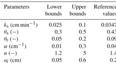
Parameters Lower Upper Reference bounds bounds values

ks(cm min−1) 0.025 0.1 0.0347

θs(−) 0.3 0.5 0.43

θr(−) 0.05 0.2 0.09

α(cm−1) 0.01 0.3 0.04

n(−) 1.2 5 1.4

al(cm) 0.05 0.6 0.2

The flow–transport model is used to analyze the effects of different measurement sets on parameter identification. For this purpose, we adopt a Bayesian approach that involves the parameter joint posterior distribution (Vrugt et al., 2008). The latter is assessed with the DREAM(ZS) MCMC sam-pler (Laloy and Vrugt, 2012). This software generates ran-dom sequences of parameter sets that asymptotically con-verge toward the target joint posterior distribution (Gelman et al., 1997). Thus, if the number of runs is sufficiently high, the generated samples can be used to estimate the statistical measures of the posterior distribution, such as the mean and variance, among other measures.

The Bayes theorem states that the probability density func-tion of the model parameters condifunc-tioned onto data can be expressed as

p (ξ|ymes)∝p (ymes|ξ ) p (ξ ) , (6)

wherep (ξ|ymes)is the likelihood function measuring how well the model fits the observations ymes, and p (ξ ) is the prior information about the parameter before the observa-tions are made. Independent uniform priors within the ranges reported in Table 1 are chosen. In this work, a Gaussian dis-tribution defines the likelihood function because the obser-vations are simulated and corrupted with Gaussian errors. Hence, the parameter posterior distribution is expressed as

p (ξ|ymes)∝exp −SSh(ξ ) 2σ_h2

−SSθ(ξ ) 2σ_θ2

−SSQ(ξ ) 2σ_Q2

−SSC(ξ ) 2σ_C2

!

, (7)

where SSh(ξ ), SSθ(ξ ), SSQ(ξ ) and SSC(ξ ) are the sums of the squared differences between the observed and mod-eled data of the pressure head, water content, cumulative outflow and output concentration, respectively. For instance, SSh(ξ )=PNk=h1

h(k)mes−h(k)mod(ξ )

2

, which includes the ob-servedh(k)mesand predictedh(k)_modpressure heads at timetkfor the number of pressure head observationsNh.

Bayesian parameter estimation is performed hereafter with the DREAM(ZS)software (Laloy and Vrugt, 2012), which is an efficient MCMC sampler. DREAM(ZS) computes multi-ple sub-chains in parallel to thoroughly explore the parame-ter space. Archives of the states of the sub-chains are stored

and used to allow a strong reduction of the “burn-in” period in which the sampler generates individuals with poor perfor-mances. Taking the last 25 % of individuals of the MCMC (when the chains have converged) yields multiple sets of pa-rameters,ξ, that adequately fit the model onto observations. These sets are then used to estimate the updated parameter distributions, the pairwise parameter correlations and the un-certainty of the model predictions. As suggested in Vrugt et al. (2003b), we consider that the posterior distribution is sta-tionary if the Gelman and Ruban (1992) criterion is≤1.2.

4 Results and discussion

In this section, the identifiability of the parameters is investi-gated for seven different scenarios of measurement sets (Ta-ble 1). In the first scenario, only measured pressure heads and cumulative outflow are used for the calibration. Scenarios 2 to 5 investigate the benefit of adding measured water contents and/or solute outlet concentrations to pressure heads and out-flow. The last scenarios (6, 7) investigate the use of mea-sured cumulative outflow and concentration breakthrough at the column outflow because these measurements do not re-quire intrusive techniques. Scenarios 5 to 7 investigate the effects of solute injection duration on the identifiability of the parameters as well.

In all cases, the MCMC sampler was run with three simul-taneous chains for a total number of 50 000 runs. Depend-ing on the scenario, the MCMC required between 5000 and 20 000 model runs to reach convergence and was terminated after 30 000 runs. The last 25 % of the runs that adequately fit the model onto observations are used to estimate the updated probability density function (pdf).

4.1 The data sets for parameter estimation

Table 2. Measurement sets and injection periods for the different scenarios. The pressure headhand the water contentθare measured at 5 cm from the top of the column. The cumulative outflowQand the concentrationCare measured at the exit of the column.

Scenario Measured variables Injection period h θ Q C Tinj=5000 min Tinj=3000 min

1 ν ν ν

2 ν ν ν ν

3 ν ν ν ν ν

4 ν ν ν ν

5 ν ν ν ν

6 ν ν ν

7 ν ν ν

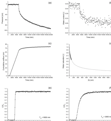
reached in the column is−120 cm, which corresponds to the initial pressure head at the top of the column.

The breakthrough concentration curve (Fig. 1e) shows a sharp front, which starts shortly after 3000 min. Note that if the injection of both water and contaminant are stopped once the solute reaches the output. For an injection period of 3000 min, the breakthrough curve exhibits a smoother pro-gression (Fig. 1f).

The data considered as measurements, which are used as conditioning information for model calibration, are also shown in Fig. 1. In Fig. 1b, the water content seems to be more affected by the perturbation of data than the pressure head and cumulative outflow. This phenomenon is due to the relative importance of the measurement errors of the wa-ter content often observed with time-domain reflectometry probes and to the weak variations of the water content dur-ing the infiltration experiment. The perturbation of the break-through curve is relatively small because of the low added noise since output concentrations can be accurately mea-sured. The perturbations of the pressure head and cumulative outflow seem weak because of the large variation of these variables during the experiment.

4.2 Results of the parameter estimation

The uncertainty model parameters are assumed to be dis-tributed uniformly over the ranges reported in Table 1. This table also lists the reference values used to generate data ob-servations before perturbation. Seven scenarios are consid-ered, corresponding to different sets of measurements for the estimation of the hydraulic and transport soil parameters (Ta-ble 2).

The MCMC results of the seven studied scenarios are given in Figs. 2–8. The “on-diagonal” plots in these fig-ures display the inferred parameter distributions, whereas the “off-diagonal” plots represent the pairwise correlations in the MCMC sample. If the draws are independent, non-sloping scatterplots should be observed. However, if a good value of a given parameter is conditioned by the value of another pa-rameter, then their pairwise scatterplot should show a narrow

sloping stripe. The sensitivity of parameters is obtained by comparing prior to posterior parameter distribution. A signif-icant difference between the two distributions for a parameter indicates high model sensitivity to that parameter (Dusek et al., 2015).

To facilitate the comparison between the different scenar-ios, Figs. 9–14 show the mean and the 95 % confidence inter-vals of the final MCMC sample that adequately fit the model onto observations for each scenario, and Table 3 summarizes the pairwise parameter correlations.

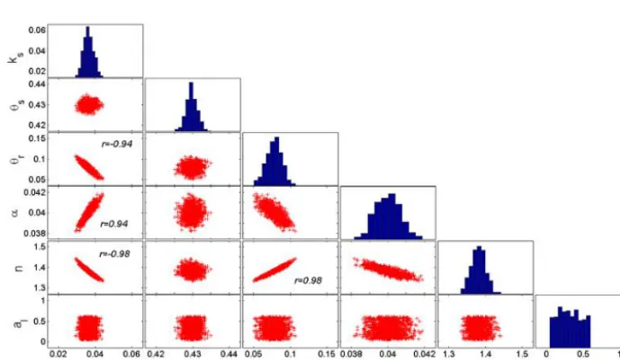
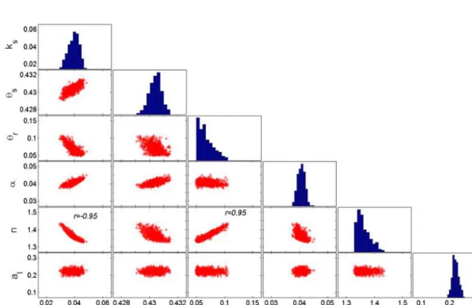
Figure 2 shows the inferred distributions of the parameters identified with the MCMC sampler using only the pressure and cumulative outflow measurements (scenario 1). The pa-rametersks,αandnare well estimated; their prior intervals of variation are strongly narrowed and they essentially show bell-shaped posterior distributions. This shows the high sen-sitivity of the model responses to these parameters.

The parameter ks is strongly correlated to α (0.94) and n (−0.97). These results confirmed the results of Eching et al. (1994) from multistep outflow experiments where it was found that the inverse solution technique is greatly im-proved when both cumulative outflow and pressure head data from some positions inside the column are used. The two water-content-related parameters are strongly correlated (0.96) and cannot be identified accurately because the wa-ter retention relationship depends on the difference between θs andθr, and only this difference is identifiable. Note that the prior intervals of θr and θs, which are, respectively, [0.05,0.2] and [0.3,0.5], have changed to the posterior inter-vals [0.05,0.16] and [0.39,0.5] because the target difference should be θs−θr=0.34. In the literature, van Genuchten and Nielsen (1985), Eching and Hopmans (1993) and Zur-mühl (1996) considered that saturated water content is deter-mined independently and considered onlyθrto be an empir-ical parameter that should be fitted to the data.

The dispersivity coefficiental has not been identified in this first scenario.

pa-Figure 1. (a)Pressure head at 5 cm below the soil surface,(b)water content at 5 cm below the soil surface,(c)cumulative outflow,(d) reten-tion curve,(e)output concentration forTinj=5000 and(f)forTinj=3000 min. Solid lines represent model outputs and dots represent the sets of perturbed data serving as conditioning information for model calibration.

Table 3.Summary of the pairwise parameter correlations.

Scenario

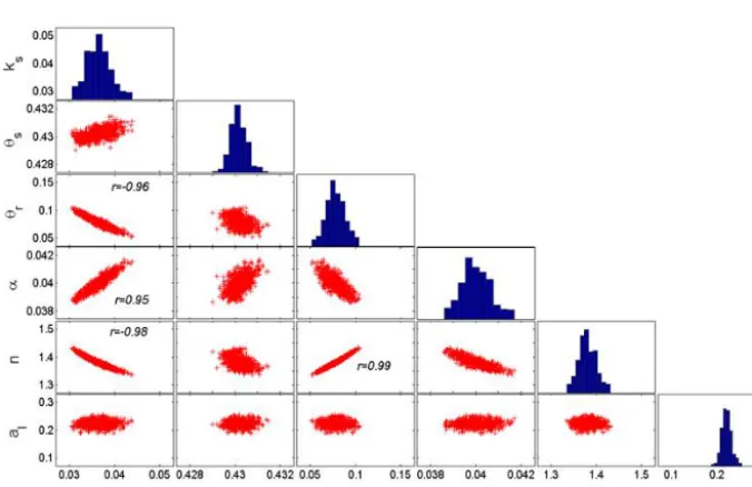
1 (ks, n)= −0.97 (ks, α)=0.94 (θr, θs)=0.96 2 (ks, n)= −0.98 (ks, α)=0.94 (ks, θr)= −0.94 (θr, n)=0.98

3 (ks, n)= −0.97 (ks, α)=0.91 (ks, θr)= −0.94 (θr, n)=0.99 4 (ks, n)= −0.98 (ks, α)=0.95 (ks, θr)= −0.96 (θr, n)=0.99 5 (ks, n)= −0.96 (ks, α)=0.93 (ks, θr)= −0.91 (θr, n)=0.98 6 (ks, n)= −0.95 (θr, n)=0.95 7 (ks, n)= −0.95 (θr, n)=0.94

rameters can be obtained with the infiltration experiment even though a limited range of water contents is covered.

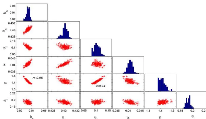
When the concentration measurements are also considered in the inversion (scenario 3), the results depicted in Fig. 4

re-Figure 2.MCMC solutions for the transport scenario 1. The diagonal plots represent the inferred posterior probability distribution of the model parameters. The off-diagonal scatterplots represent the pairwise correlations in the MCMC drawing.

Figure 3.MCMC solutions for transport scenario 2 (see Fig. 2 caption).

duced, leading to a good identification of these parameters when usingCmeasurements (Figs. 10 and 14). A better es-timate of the saturated water content is obtained because ad-vective transport is a function of this variable.

In the inversion procedure of scenario 4, the measurements of the water content are not considered. This scenario leads to the same quality of the estimation for the parametersks, θr,αandn(Figs. 9, 11, 12, 13) and similar correlations be-tween the parameters as in the previous scenario. This result shows that the intrusive water content measurements, which are subject to more significant measurement errors than the output concentration, are not required if the output concen-tration is measured. Compared with the results of scenario 2,

it can be concluded that better parameter estimations are ob-tained usingh,QandC data than usingh,Qandθ data, especially forθs. Therefore, usingC instead ofθ measure-ments in combination withh and Qmeasurements allows the estimation ofal and yields a better estimate ofθs.

un-Figure 4.MCMC solutions for transport scenario 3 (see Fig. 2 caption).

Figure 5.MCMC solutions for transport scenario 4 (see Fig. 2 caption).

certainty of these parameters is smaller because the credible interval is reduced by a factor of 25 % forks, 8 % forθs, 26 % forθr, 10 % forαand 25 % fornwhen compared to the re-sults obtained usingTinj=5000 min. The parameteralis also much better estimated than in the previous scenario. Its mean value approaches the reference solution and the posterior un-certainty range is reduced by approximately 75 % (Fig. 14).

In scenario 6, the pressure head measurements are re-moved and only non-intrusive measurements (QandCdata) are used for the calibration with an injection period of Tinj=5000 min. These kinds of non-intrusive measures have been used by Mertens et al. (2009) to estimate some of the hydraulic and pesticide leaching parameters. The results

Figure 6.MCMC solutions for transport scenario 5 (see Fig. 2 caption).

Figure 7.MCMC solutions for transport scenario 6 (see Fig. 2 caption).

of the parameterαis similar to that in scenario 4. However, its uncertainty is much larger because the credible interval is 77 % larger (Fig. 14). The parametersθsandalare estimated as well as in scenario 4 (in terms of mean estimated value and credible interval).

The last scenario (scenario 7) is similar to the previous one, but the injection period is reduced toTinj=3000 min. The results depicted in Fig. 8 show similar correlations between the parameters as for Tinj=5000 min. However, a significant improvement is observed for the mean esti-mated values, which approach the reference solution for ks, θr, n and al (Figs. 9, 11, 13, 14). The uncertainties

Figure 8.MCMC solutions for transport scenario 7 (see Fig. 2 caption).

Figure 9.Posterior mean values and 95 % confidence intervals of the saturated hydraulic conductivity for the different scenarios.

in Fig. 1c). As a consequence, the concentration profile in-creases smoothly (see Fig. 1f) until reaching its maximum value, in contrast to the sharp front observed for Tinj= 5000min in scenario 6 (see Fig. 1e). Hence, the breakthrough curve obtained withTinj=3000 min is more affected by the hydraulic parameters than the breakthrough curve obtained withTinj=5000 min. This explains why a better estimation of the parameters is observed for the last scenario compared to scenario 6.

5 Conclusions

In this work, estimation of hydraulic and transport soil pa-rameters have been investigated using synthetic infiltration

Figure 10.Posterior mean values and 95 % confidence intervals of the saturated water content for the different scenarios.

experiments performed in a column filled with a sandy clay loam soil, which was subjected to continuous flow and solute injection over a periodTinj.

The saturated hydraulic conductivity, the saturated and residual water contents, the Mualem–van Genuchten shape parameters and the longitudinal dispersivity are estimated in a Bayesian framework using the MCMC sampler. Parameter estimation is performed for different scenarios of data mea-surements.

The results reveal the following conclusions:

Figure 11.Posterior mean values and 95 % confidence intervals of the residual water content for the different scenarios.

Figure 12.Posterior mean values and 95 % confidence intervals of the shape parameterαfor the different scenarios.

Tinj, even if the water content remains close to saturated conditions.

2. The use of concentration measurements at the column outflow, in addition to traditional measured variables (water content, pressure head and cumulative outflow), reduces the hydraulic parameter uncertainties, espe-cially those of the saturated water content (comparison between scenarios 2 and 3).

3. The saturated hydraulic conductivity is estimated with the same order of accuracy, independent of the observed variables.

4. The estimation of the dispersivity is sensitive to the in-jection duration. Scenarios 5 and 7 withTinj=3000 min yield much more accurate dispersivity estimations than scenarios 4 and 6 with Tinj=5000 min due to

Figure 13.Posterior mean values and 95 % confidence intervals of the shape parameternfor the different scenarios.

Figure 14.Posterior mean values and 95 % confidence intervals of dispersivity for the different scenarios.

the extended spreading of the solute observed for Tinj=3000 min.

5. A better identifiability of the soil parameters is obtained usingCinstead ofθmeasurements, in combination with handQdata (comparison between scenarios 2 and 4). 6. Using only non-intrusive measurements (cumulative

in soils. The setup has to be appropriately equipped to mea-sure the cumulative water outflow (e.g., weighing machine) and the solute breakthrough at the column outflow (e.g., flow through electrical conductivity). The injection should be stopped as soon as the solute concentration reaches the out-flow. The accuracy of the estimation ofθr,αandnimproves by adding pressure measurements inside the column, close to the injection.

These results are of course related to the models and ex-perimental conditions we used. This work can be extended to different types of soils, water retention and/or relative per-meability functions to evaluate the interest of coupling flow and transport for parameter identification. This work can also be extended to reactive solutes.

Data availability. No data sets were used in this article.

Competing interests. The authors declare that they have no conflict of interest.

Acknowledgements. The authors are grateful to the French

National Research Agency, which funded this work through the program AAP Blanc – SIMI 6 project RESAIN (no. ANR-12-BS06-0010-02).

Edited by: H. Cloke

Reviewed by: four anonymous referees

References

Ades, A. E. and Lu, G.: Correlations between parameters in risk models: estimation and propagation of uncertainty by Markov Chain Monte Carlo, Risk Anal., 23, 1165–1172, 2003.

Carrera, J. and Neuman, S. P.: Estimation of aquifer parameters un-der transient and steady conditions: 2. Uniqueness, stability and solution algorithms, Water Resour. Res., 22, 211–227, 1986. Durner, W. and Iden, S. C.: Extended multistep outflow method

for the accurate determination of soil hydraulic properties near water saturation, Water Resour. Res., 47, W08526, doi:10.1029/2011WR010632, 2011.

Durner, W., Schultze, B., and Zurmühl, T.: State-of-the-art in in-verse modeling of inflow/outflow experiments, edited by: Van Genuchten, M. T., Leij, F. J., and Wu, L., in: Characterization and Measurement of the Hydraulic Properties of Unsaturated Porous Media, Proc. Int. Worksh., Riverside, CA, University of Califor-nia, Riverside, 661–681, 1999.

Dusek, J., Dohnal, M., Snehota, M., Sobotkova, M., Ray, C., and Vogel, T.: Transport of bromide and pesticides through an undisturbed soil column: a modeling study with global optimization analysis, J. Contam. Hydrol., 175–176, 1–16, doi:10.1016/j.jconhyd.2015.02.002, 2015.

Eching, S. O. and Hopmans, J. W.: Optimization of hydraulic func-tions from transient outflow and soil water pressure data, Soil Sci. Soc. Am. J., 57, 1167–1175, 1993.

Eching, S. O., Hopmans, J. W., and Wendroth, O.: Unsaturated Hydraulic Conductivity from Transient Multistep Outflow and Soil Water Pressure Data, Soil Sci. Soc. Am. J., 58, 687–695, doi:10.2136/sssaj1994.03615995005800030008x, 1994. Fahs, M., Younes, A., and Lehmann, F.: An easy and efficient

com-bination of the Mixed Finite Element Method and the Method of Lines for the resolution of Richards’ Equation, Environ. Modell. Soft., 24, 1122–1126, doi:10.1016/j.envsoft.2009.02.010, 2009. Fahs, M., Younes, A., and Ackerer, P.: An efficient

imple-mentation of the method of lines for multicomponent reac-tive transport equations, Water Air Soil Poll., 215, 273–283, doi:10.1007/s11270-010-0477-y, 2011.

Farthing, M. W., Kees, C. E., and Miller, C. T.: Mixed finite element methods and higher order temporal approximations for variably saturated groundwater flow, Adv. Water Resour., 26, 373–394, doi:10.1016/S0309-1708(02)00187-2, 2003.

Gallagher, M. and Doherty, J.: Parameter estimation and uncertainty analysis for a watershed model, Environ. Modell. Softw., 22, 1000–1020, doi:10.1016/j.envsoft.2006.06.007, 2007.

Gelman, A. and Rubin, D. B.: Inference from iterative simulation using multiple sequences, Stat. Sci., 7, 457–472, 1992.

Gelman, A., Carlin, J. B., Stren, H. S., and Rubin, D. B.: Bayesian data analysis, Chapmann and Hall, London, 1997.

Hopmans, J. W., Simunek, J., Romano, N., and Durner, W.: Simul-taneous determination of water transmission and retention prop-erties, Inverse Methods, edited by: Dane, J. H. and Topp, G. C., Methods of Soil Analysis. Part 4. Physical Methods, Soil Science Society of America Book Series No. 5, 963–1008, 2002. Hudson, D. B., Wierenga, P. J., and Hills, R. G.: Unsaturated

hy-draulic properties from upward flow into soil cores, Soil Sci. Soc. Am. J., 60, 388–396, 1996.

Inoue, M., Šim˚unek, J., Hopmans, J. W., and Clausnitzer, V.: In situ estimation of soil hydraulic functions using a multistep soil-water extraction technique, Water Resour. Res., 34, 1035–1050, 1998.

Inoue, M., Šim˚unek, J., Shiozawa, S., and Hopmans, J. W.: Simul-taneous estimation of soil hydraulic and solute transport param-eters from transient infiltration experiments, Adv. Water Resour., 23, 677–688, doi:10.1016/S0309-1708(00)00011-7, 2000. Kahl, G. M., Sidorenko, Y., and Gottesbüren, B.: Local and global

inverse modelling strategies to estimate parameters for pesticide leaching from lysimeter studies, Pest Manag. Sci., 71, 616–631, doi:10.1002/ps.3914, 2015.

Kool, J. B. and Parker, J. C.: Analysis of the inverse problem for transient unsaturated flow, Water Resour. Res., 24, 817–830, 1988.

Kool, J. B., Parker, J. C., and van Genuchten, M. T.: Determining soil hydraulic properties from one-step outflow experiments by parameter estimation: I. Theory and numerical studies, Soil Sci. Soc. Am. J., 49, 1348–1354, 1985.

Laloy, E. and Vrugt, J. A.: High-dimensional posterior explo-ration of hydrologic models using multiple-try DREAM(ZS) and high-performance computing, Water Resour. Res., 48, W01526, doi:10.1029/2011WR010608, 2012.

Richards’ equation, Adv. Water Resour., 30, 555–575, doi:10.1016/j.advwatres.2006.04.011, 2007.

Marquardt, D. W.: An algorithm for least-squares estimation of non-linear parameters, SIAM J. Appl. Math., 11, 431–441, 1963. Mertens, J., Kahl, G., Gottesbüren, B., and Vanderborght, J.:

Inverse Modeling of Pesticide Leaching in Lysimeters: Lo-cal versus Global and Sequential Single-Objective versus Multiobjective Approaches, Vadose Zone J., 8, 793–804, doi:10.2136/vzj2008.0029, 2009.

Miller, C. T., Williams, G. A., Kelly, C. T., and Tocci, M. D.: Robust solution of Richards’ equation for non uniform porous media, Water Resour. Res., 34, 2599–2610, doi:10.1029/98WR01673, 1998.

Miller, C. T., Abhishek, C., and Farthing, M.: A spatially and tem-porally adaptive solution of Richards’ equation, Adv. Water Re-sour., 29, 525–545, doi:10.1016/j.advwatres.2005.06.008, 2006. Mishra, S. and Parker, J. C.: Parameter estimation for coupled un-saturated flow and transport, Water Resour. Res., 25, 385–396, doi:10.1029/WR025i003p00385, 1989.

Mualem, Y.: A new model for predicting the hydraulic conductivity of unsaturated porous media, Water Resour. Res., 12, 513–522, doi:10.1029/WR012i003p00513, 1976.

Nasta, P., Huynh, S., and Hopmans, J. W.: Simplified Multistep Out-flow Method to Estimate Unsaturated Hydraulic Functions for Coarse-Textured, Soil Sci. Soc. Am. J., 75, p. 418, 2011. Šim˚unek, J. and van Genuchten, M. T.: Estimating unsaturated

soil hydraulic properties from multiple tension disc infiltrome-ter data, Soil Sci., 162, 383–398, 1997.

Tocci, M. D., Kelly, C. T., and Miller, C. T.: Accurate and eco-nomical solution of the pressure-head form of Richards’ equa-tion by the method of lines, Adv. Water Resour., 20, 1–14, doi:10.1016/S0309-1708(96)00008-5, 1997.

van Dam, J. C., Stricker, J. N. M., and Droogers, P.: Inverse method for determining soil hydraulic functions from one-step outflow experiment, Soil Sci. Soc. Am. J., 56, 1042–1050, 1992. van Dam, J. C., Stricker, J. N. M., and Droogers, P.: Inverse

method to determine soil hydraulic functions from multistep outflow experiments, Soil Sci. Soc. Am. J., 58, 647–652, doi:10.2136/sssaj1994.03615995005800030002x, 1994.

van Genuchten, M. T.: A closed form equation for predicting the hydraulic conductivity of unsaturated soils, Soil Sci. Soc. Am. J., 44, 892–898, doi:10.2136/sssaj1980.03615995004400050002x, 1980.

van Genuchten, M. T. and Nielsen, D. R.: On describing and pre-dicting the hydraulic properties of unsaturated soils, Ann. Geo-phys., 3 615–628, 1985.

Vrugt, J. A. and Bouten, W.: Validity of first-order approximations to describe parameter uncertainty in soil hydrologic models, Soil. Sci. Soc. Am. J., 66, 1740–1751, doi:10.2136/sssaj2002.1740, 2002.

Vrugt, J. A., Bouten, W., Gupta, H. V., and Hopmans, J. W.: To-ward improved identifiability of soil hydraulic parameters: On the selection of a suitable parametric model, Vadose Zone J., 2, 98–113, doi:10.2113/2.1.98, 2003a.

Vrugt, J. A., Gupta, H. V., Bouten, W., and Sorooshian, S.: A shuffled complex evolution Metropolis algorithm for optimiza-tion and uncertainty assessment for hydrologic model parame-ters, Water Resour. Res., 39, 1201, doi:10.1029/2002WR001642, 2003b.

Vrugt, J. A., ter Braak, C. J. F., Clark, M. P., Hyman, J. M., and Robinson, B. A.: Treatment of input uncertainty in hy-drologic modeling: Doing hydrology backward with Markov chain Monte Carlo simulation, Water Resour. Res., 44, W00B09, doi:10.1029/2007WR006720, 2008.

Younes, A., Fahs, M., and Ahmed, S.: Solving density driven flow problems with efficient spatial discretizations and higher-order time integration methods, Adv. Water Resour., 32, 340–352, doi:10.1016/j.advwatres.2008.11.003, 2009.

Younes, A., Mara, T. A., Fajraoui, N., Lehmann, F., Belfort, B., and Beydoun, H.: Use of Global Sensitivity Analysis to Help Assess Unsaturated Soil Hydraulic Parameters, Vadose Zone J., 12, 1– 12, doi:10.2136/vzj2011.0150, 2013.