The Validity Analysis of Regression: Combining Uniform Experiment Design with Nonlinear Regression

http://dx.doi.org/10.4236/am.2015.66092

How to cite this paper: Yang, N., Zhang, D.W. and Tian, Y.L. (2015) The Validity Analysis of Regression: Combining Uniform Experiment Design with Nonlinear Regression. Applied Mathematics, 6, 996-1008.

http://dx.doi.org/10.4236/am.2015.66092

The Validity Analysis of Regression:

Combining Uniform Experiment

Design with Nonlinear Regression

Nan Yang

1,2*

, Dawei Zhang

1

, Yanling Tian

1

1_{School of Mechanical Engineering, Tianjin University, Tianjin, China}

2_{Tianjin Key Laboratory of the Design and Intelligent Control of the Advanced Mechatronical System, School of}

Mechanical Engineering, Tianjin University of Technology, Tianjin, China Email: *_{[email protected]}

Received 27 March 2015; accepted 2 June 2015; published 5 June 2015

Copyright © 2015 by authors and Scientific Research Publishing Inc.

This work is licensed under the Creative Commons Attribution International License (CC BY).

http://creativecommons.org/licenses/by/4.0/

Abstract

The data topology structure of uniform experiment design (UD) is too complex to be reasonable regressed. In this paper, the principle and method of distinguish the training data and testing data were described to make a reasonable regression when uniform experiment design combined with support vector regression (SVR). Two equivalent ways which were the smallest enclosing hyper-sphere perceptron (SEH) and the enclosing simplex perceptron (ES) were provided to discover the topology relationship of the process parameter datum. To give an application, a series of experi-ments about laser cladding layer quality were conducted by UD to get the relationship of load, ve-locity and wearing capacity. Results showed that only the testing datum recommended by the two perceptrons got a good forecasting by SVR. Therefore, the two perceptrons could guide experi-ments with process parameter data of complex topology structure. Further, the application could be extended over a much wider field of experiments.

Keywords

Uniform Experiment Design, Support Vector Machine, The Smallest Enclosing Hyper Sphere, The Enclosing Simplex

1. Introduction

Many researches focus on experimental design combining with nonlinear regression. The experiment design

method includes uniform design, central composite experimental design and Taguchi’s approach; the nonlinear regression method includes artificial neural network, support vector machine and so on. Some focus on the ex-perimental design optimizing the nonlinear regression parameters; others focus on the nonlinear regression op-timizing the experimental design to get the best process parameters under the desired results.

Yanwei Li et al. [1] used uniform design optimized support vector machine to be an experimental guide to find macrocyclic compounds which were used to detect and minimize the radiocesium pollution. Weihong Li et al. [2] proposed a multi-objective uniform design search method as a SVM model selection tool, and applied this optimized SVM classifier to face recognition. Xiaolin Yu [3] used uniform design and least support vector ma-chines method for reliability analysis of large complex structures. Guangya Zhang [4] used support vector ma-chine to develop the non-linear quantitative structure-property relationship model of the G/11 xylanase based on the amino acid composition, and used the uniform design to optimize the running parameters of SVM. Ni L.J. [5] improved v-support vector machines method to build classification models for discriminating adulteration milks based on near infrared spectra of different sample sets, and used uniform design table to find good value of pa-rameters of v and sigma. Xiaolin Yu et al. [6] proposed the reliability analysis method based on uniform design method and supported vector machine to get the failure probability. A joint optimization method is proposed by Changsheng Xiang et al. [7] for phase space reconstruction and least square support vector machine parameters. The phase space reconstruction and least squares support vector machine parameters are jointly designed using uniform design. Wang Zhi-ming et al. [8] developed a small-scale search method based on uniform design using support vector regression. Chuang S.C. et al. [9] realized that one found many non-rectangular types of input domains on which traditional UD methods could not be adequately applied when conducting a typical computer experiment, and proposed a new UD method that was suitable for design area. Pan Jinshui et al. [10] investi-gated the possibility of optimizing mammalian cells transfection efficiency by using a method referred to as least-squares support vector machine, which required only a few experiments based on UD to maintain fairly high accuracy. Xiao Wang et al. [11] used the central composite rotatable experimental design combining with the artificial neural network (ANN) to establish the relationships among the laser power, velocity, clamp pres-sure, joint strength, and joint width. 30 experiments were conducted based on four factors five-level design. Yuwen Sun et al. [12], focused on the influence of laser power, scanning speed and powder feed rate on the shape factor and the cladding bead geometry (layer width, layer height and molten depth) with regard to inject-ing Ti6Al4V powder on TC4 substrate. Response surface methodology was used to build the mathematical model.

Dongxia Yang et al. [13], carefully selected the laser welding parameters of laser power, welding speed and wire feed rate to produce a weld joint with the minimum weld bead width and the fusion zone area. Taguchi approach was used as a statistical design of experimental technique for optimizing the parameters. They found that the ef-fect of welding parameters on the welding quality decreased in the order of welding speed, wire feed rate, and laser power. They also found the optimal combination of welding parameters. H. Beygi et al. [14], fabricated Ni coated aluminum nanoparticles by electroless nickel deposition. Effect of two groups of parameters on the process plating rate were investigated: bath composition (main salt, reducing agent and complexing agent con-centration) and process parameters (pH, plating time and bath temperature). Simulation of the process was per-formed using ANN. It was based on the ANN model to design a high efficiency electroless bath, while minimum received materials were used and maximum plating rate was obtained. Wang Zhifei et al. [15] proposed an opti-mization design scheme based on orthogonal testing and support vector machines to get relationships between each parameter and product quality features. Orthogonal testing design was used to estimate the appropriate ini-tial value and variation domain of each variable to decrease the number of iterations and improve the identifica-tion accuracy and efficiency.

However, an important step has been neglected in existing research, which is the regression validity. The searching point might go out of the experimental domain, which is not obvious to know. So the searching point will find a bad forecasting value on the regression surface, particularly when the process parameters arranged by the experimental design have complex topology boundary, for example the uniform design.

2. Principle

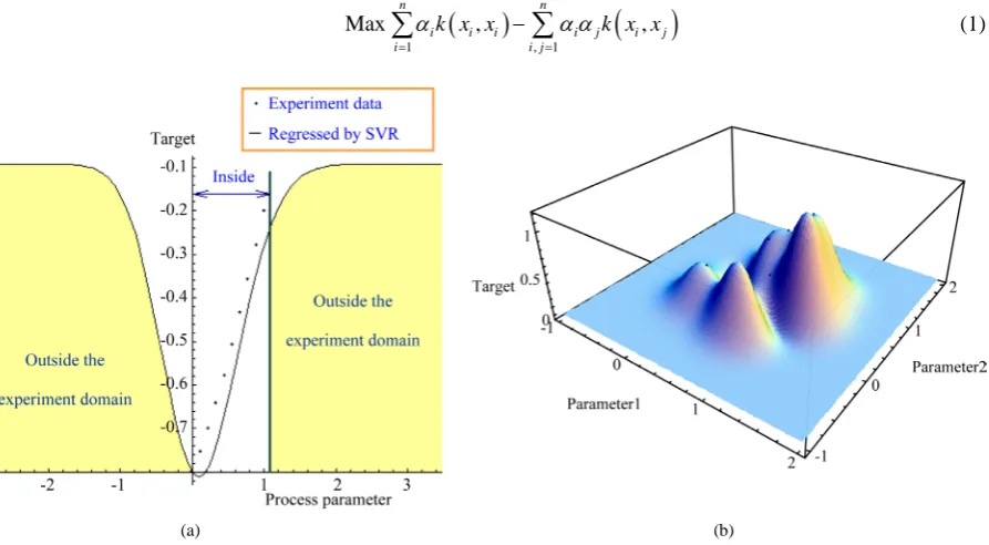
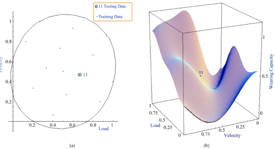
The process parameter vector should be inside the domain of the experiment, if not, the forecasting is not rea-sonable because of data absence. For example, inFigure 1(a)), 10 experiment data are regressed by SVR (hori-zontal axis is process parameter, and vertical axis is the target), the curve goes hori(hori-zontally towards a constant value outside the experiment domain, which is exactly the constant b of the pattern function of SVR (Equation (9)). For two-dimension case, inFigure 1(b)), the SVR surface gives good forecast only above the parameter 1- parameter 2 plane where the experimental data exist, whereas SVR surface keeps constant in other place.

Should the forecasting value always be constant outside the experiment data space because we do not do the experiment? Certainly, no. So, the SVR forecasts well within the experiment data space, while it could not fore-cast the outside of the experiment data space.

The forecasting is false outside the experiment domain by SVR. The curve/surface goes horizontally towards a constant value (which is the constant b (Equation (9)) of the pattern function of SVR) outside the experiment domain and causes a false forecasting.

Although distinguishing the inside and outside of the experiment data space is easy in one-dimension (only one parameter inFigure 1), the task in higher dimension (two or above) is not so easy. Therefore, the method for higher dimension is elaborated below.

2.1. The Task: Distinguishing the Training Data and Testing Data

In this paper, the task is to distinguish the training data and the testing data among lots of experimental data when the experiment is conducted by UD. The key point is whether the testing data lie inside the training data domain or not, because the function of regression is generated by the training data. So, if the testing data lie out-side the training data domain, the regression is not reasonable because of data insufficiency.

Two equivalent perceptrons are provided to discover this topology relationship in higher dimension of para-meter space. They are the smallest enclosing hypersphere (SEH) perceptron and the enclosing simplex (ES) perceptron.

2.1.1. The SEH Perceptron

The SEH in a feature space defined by a kernel k enclosing a dataset

{

x₁,,x_n

}

is computed by finding α* as solution of the optimization problem:

(

)

(

)

1 , 1

Max , ,

n n

i i i i j i j

i i j

k x x k x x

α α α

= =

−

∑

∑

(1)

[image:3.595.93.540.452.698.2]

(a) (b)

1

s.t. 1, 0, 1, ,

n

i i

i

i n

α α

=

= ≥ =

∑

 (2)

The pattern function is:

( )

( )

*

(

)

, 2 i , i

i

f x =k x x −

∑

α

k x x +d (3)

where:

(

)

(

)

* * *

, 1 1

2 , ,

n n

i j i j i i i

i j i

d α α k x x α k x x

= =

=

∑

−

∑

(4)

And k is a radical base kernel:

(

)

(

2 2

)

, exp

k x x′ = − −x x′

δ

(5)

where δ is Gauss parameter. So, calculate Equation (3), if f x

( )

<0, then x lies inside the SEH, if f x

( )

>0, then x lies outside the SEH, specially, x lies on the SEH edge with f x

( )

=0. The SEH is not a “pure round sphere” shape; it can adapt the data “shape” automatically.

2.1.2. The ES Perceptron

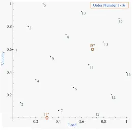
[image:4.595.75.537.84.256.2]

Another simple method could judge whether a point lies inside or outside a point set. A point inside the speci-men point set should be enclosed in the simplex consisted of n closest points. In s dimension space, n equals to s + 1. For example, in 2D space, an internal point should be enclosed by the 3 closest points (for example, in Figure 2, point 18 is enclosed by point 8, 11, 13), while an external one do not (for example, point 17 is not in the triangle of the 3 closest points 2, 4, 7).

Generally, in s dimension space, there are s + 2 determinants about a point X* =

(

x₁,,xs

)

and its s + 1 closest points: Xi =

(

x_1,i,,xs i_,

)

, i=1,,s+1:

[image:4.595.183.445.417.673.2]

11 1 1

12 2 12 2

1,2, , 1 *,2, , 1

1, 1 , 1 1, 1 , 1

11 1 11 1

1 12 2

1,*, , 1 1,2, ,*

1, 1 , 1 1

1 1 1 1 , , , 1 1 1 1 1 1 1 1 , 1 1 1 1 s s s s s s

s s s s s s

s s

s s

s

s s s s

x x x x

x x x x

D D

x x x x

x x x x

x x x x

D D

x x x x

+ + + + + + + + + = = = =                              (6)

If D_1,2,,s+1⋅D_*,2,,s+1≥0, D_1,2,,s+1⋅D_1,*,,s+1≥0, ⋅⋅⋅, and D_1,2,,s+1⋅D_1,2,,*≥0 are simultaneously true, then point X* is an internal point, otherwise, it is an external point.

The distance L between two points X X₁, ₂ is defined as:

1 2

L= X −X (7)

2.1.3. Comparison of the Two Perceptron

The ES perceptron includes distance calculation, reorder, and determinant calculation, while the SEH perceptron iterates depend on 3 artificial parameters (δ , iteration step length and iterations), so, ES is objective and fast, the most important, the region determined by ES is smaller than SEH.

2.2. Regression of SVR

Considering a training dataset:

(

)

(

)

{

1, 1 , , ,

}

(

)

, , , 1, , .

n s

n n i i

T = x y  x y ∈ X Y× x ∈X =R y ∈ =Y R i=  n

Choosing parameter ε and kernel k to solute the optimization problem:

(

)

(

) (

)

(

)

(

)

, 1 1 1

1

Min ,

2

n n n

i i j j i j i i i i i

i j i i

k x x y

β α β α ε β α β α

= = =

− − + + − −

∑

∑

∑

(8)

(

)

1

s.t. 0, 0, 0, 1, ,

n

i i i i

i

i n

β α β α

=

− = ≥ ≥ =

∑

 (9)

With the optimization solution *_, *_{, 1, ,}

i i i n

β α =  , the pattern function is:

( )

(

* *

)

(

)

1

,

n

i i i

i

g x β α k x x b

=

=

∑

− + (10)

(

* *

) (

)

1

,

n

j i i i j

i

b y β α k x x ε

=

= −

∑

− − (11)

where

α

*j>0, the corresponding support vector is

(

x yj, j

)

. And k is also a radical base kernel as shown in Equation (5), g(x)is the regression target function.

SVR could get a nonlinear regression function g(x) based on a training dataset without artificial judgment of the function power ahead of time. And the training dataset is recommended by the SEH or ES perceptron.

3. Experiment

func-tion. The SEH or ES perceptron is used to distinguish the testing data from the training data among all the process parameters.

A laser cladding layer quality forecasting experiment is conducted for a clear view of the principle. We coat the Ni-based alloy on the CrMo in order to develop the resistance to wear of the substrate material via laser cladding process. The experiment task is to get wearing capacity under the variety of the combinations of the load (the pressure to the material) and the loading velocity (the velocity of moving the material). So, in this ex-periment, we have two experimental factors (process parameters): load and velocity, and the experimental target is wearing capacity.

The levels number of the load and velocity could be given as any natural number you want, and it means that you should do much more experiments if the levels number is higher. When the experiment factors and levels are determined, the experiment could be arranged by UD table and its application table which could be known in Ref. [16].

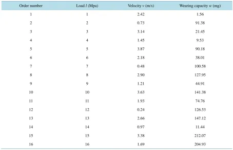
Here, the levels are given as 16, so, it means that we need only 16 experiments (orthogonal experiment needs 162 = 256 experiments). The levels of the load and velocity are respect 1 - 16 Mpa and 0.24 - 3.87 m/s. The combination of the two parameters and corresponding experimental results are listed inTable 1.

4. Results and Discussion

The wearing capacity varies with different load and velocity, so the regression aim is to obtain the function: wearing capacity = f (load, velocity). But it is troublesome that the domain is not in good order. If the testing data we choose lie outside of the domain, the testing data is invalid. Here, we use the SEH or ES perceptron to judge whether the testing data lie inside the domain or not.

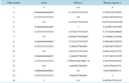
Firstly, the process parameters are normalization. The corresponding nondimensional quantities are shown in Table 2, which are arranged by unitary processing blow.

min

max min

p p

u

p p

− =

[image:6.595.85.540.430.724.2]

− (12)

Table 1.The processing parameters (load and velocity) and experimental results (wearing capacity) based on UD.

Order number Load l (Mpa) Velocity v (m/s) Wearing capacity w (mg)

1 1 2.42 1.56

2 2 0.73 91.38

3 3 3.14 21.45

4 4 1.45 9.53

5 5 3.87 90.18

6 6 2.18 38.01

7 7 0.48 100.58

8 8 2.90 127.95

9 9 1.21 44.91

10 10 3.63 141.38

11 11 1.93 74.76

12 12 0.24 126.53

13 13 2.66 147.12

14 14 0.97 11.44

15 15 3.38 212.07

[image:7.595.86.537.101.391.2]

Table 2.The nondimensional processing parameters and experimental results.

Order number Load l Velocity v Wearing capacity w

1 0 0.6 0

2 0.0666666666666667 0.133241379310345 0.426705301159035

3 0.133333333333333 0.8 0.0945278358350751

4 0.2 0.333241379310345 0.0379218126543796

5 0.266666666666667 1 0.421005130153905

6 0.333333333333333 0.533241379310345 0.173142694280828

7 0.4 0.0664827586206897 0.470406612198366

8 0.466666666666667 0.733241379310345 0.600418012540376

9 0.533333333333333 0.26648275862069 0.205918677560327

10 0.6 0.933241379310345 0.664212426372791

11 0.666666666666667 0.46648275862069 0.347710431312939

12 0.733333333333333 1.95904116683588E−18 0.593767813034391

13 0.8 0.66648275862069 0.69147824434733

14 0.866666666666667 0.2 0.04678890366711

15 0.933333333333333 0.86648275862069 1

16 1 0.4 0.965941478244347

where p is given process parameter, pmin and pmax are the minimum and maximum of p, and u is the unitary

processing result. The 16 load-velocity 2D points are shown inFigure 2, where 17 and 18 represent new expe-riments which will be discussed later.

The strategies described in this paper have been implemented in Delphi package, and the artificial parameters for SEH are given as:δ2 = 0.5, iteration step length = 0.01, iterations = 100000.There are no artificial parame-ters for ES.

4.1. The SEH Perceptron

If the training data and testing data are chosen randomly (among the 16 points), the testing data might lie outside the training data, so the regression analysis is invalid. For example, if point 15 (an edge point)is chosen as the testing data and the remain as the training data, it is found that point 15 lies outside the training data, and this could be felt by the SEH perceptron, as shown inFigure 3. Point 15 could not get an effective forecasting value, because the curve surface collapses without any support data.

However, if an internal point is chosen as the testing data, the situation will be changed. As shown inFigure 4, point 11 is an internal point, so, it is circled in the SEH. The forecasting result is also good, the 3D point is al-most on the surface which is regressed by point 1 to 16 not include 11, the error between the forecasting value and the testing value is small as shown inTable 3. Furthermore, the surface regressed by point 1 to 16 (the re-gression error is shown inTable 4) agrees perfectly with the surface regressed by point 1 to 16 excluding point 11 inFigure 5(a), that is to say point 11 don’t affect the regression surface. The contour of regression surface is shown inFigure 5(b), from which we can see that a low velocity with a high load or a high velocity with a low load may cause a low wear capacity.

[image:8.595.87.538.84.338.2]

(a) (b)

Figure 3.Point 15 is chosen as testing datum and the rest are training data, so the SVR is fail to forecast point 15 via 3D re-gression surface. (a) Point 15 lies outside the SHE; (b) Point 15 is far away from the 3D rere-gression surface.

(a) (b)

Figure 4. Point 11 is chosen as a testing datum and the rest are training data, so the SVR forecasts point 11 via 3D regression surface successfully. (a) Point 11 lies inside the SHE; (b) Point 11 agrees with the regression surface.

[image:8.595.94.539.372.613.2]

[image:9.595.88.540.102.404.2]

Table 3.The comparison of the regressive value and experimental value, 11 is testing datum while the rest are training data.

Category Order number Regressive value Experimental value Error

Training data

1 9.99999999998066E−5 0 9.99999999998066E−5

2 0.426605301159035 0.426705301159035 0.000100000000000194

3 0.0946278358350749 0.0945278358350751 9.9999999999808E−5

4 0.0380218126543794 0.0379218126543796 9.9999999999808E−5

5 0.420905130153904 0.421005130153905 0.000100000000000193

6 0.173242694280828 0.173142694280828 9.99999999998061E−5

7 0.470506612198366 0.470406612198366 9.99999999998062E−5

8 0.600318012540376 0.600418012540376 0.000100000000000191

9 0.205818677560327 0.205918677560327 0.000100000000000193

10 0.664312426372791 0.664212426372791 9.99999999998063E−5

12 0.593667813034391 0.593767813034391 0.000100000000000191

13 0.69157824434733 0.69147824434733 9.9999999999804E−5

14 0.0468889036671098 0.04678890366711 9.99999999998016E−5

15 0.9999 1 0.0001

16 0.965841478244347 0.965941478244347 0.000100000000000188

Testing data 11 0.290105323107535 0.347710431312939 0.057605108205404

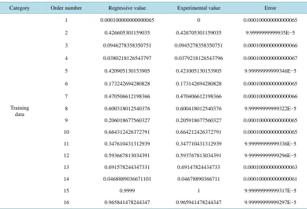
Table 4. The comparison of the regressive value and experimental value, all points are training data.

Category Order number Regressive value Experimental value Error

Training data

1 0.000100000000000065 0 0.000100000000000065

2 0.426605301159035 0.426705301159035 9.9999999999935E−5

3 0.0946278358350751 0.0945278358350751 0.000100000000000066

4 0.0380218126543797 0.0379218126543796 0.000100000000000067

5 0.420905130153905 0.421005130153905 9.99999999999346E−5

6 0.173242694280828 0.173142694280828 0.000100000000000065

7 0.470506612198366 0.470406612198366 0.000100000000000066

8 0.600318012540376 0.600418012540376 9.99999999999322E−5

9 0.206018677560327 0.205918677560327 0.000100000000000065

10 0.664312426372791 0.664212426372791 0.000100000000000065

11 0.347610431312939 0.347710431312939 9.99999999999336E−5

12 0.593667813034391 0.593767813034391 9.99999999999296E−5

13 0.691578244347331 0.69147824434733 0.000100000000000063

14 0.0468889036671101 0.04678890366711 0.000100000000000061

15 0.9999 1 9.99999999999317E−5

[image:9.595.92.538.416.719.2]

[image:10.595.89.540.81.294.2]

(a) (b)

Figure 5. The meshed surface is regressed by point 1-16, while the unmeshed one is regressed by point 1-16 except 11. The two surfaces agree with each other very well. The minimum of wearing capacity could be found from the contour map. (a)

[image:10.595.188.434.342.546.2]

The regression surface; (b) Contour map of the regression surface.

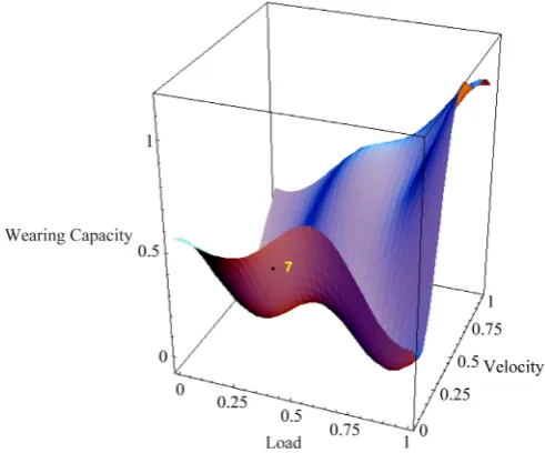
Figure 6.Successful forecasting of point 7. Point 7 is an edge point

but also inside the SEH, so, it could be well forecasted.

4.2. The ES Perceptron

If point 5 is chosen as a testing datum, the three closest points are 3, 8, 10, (Figure 2) and then calculate the de-terminants:

3 3 5 5

3,8,10 8 8 5,8,10 8 8

10 10 10 10

1 1

1 0.075 0, 1 0.075 0

1 1

v l v l

D v l D v l

v l v l

= = > = = >

3 3 3 3

3,5,10 5 5 3,8,5 8 8

10 10 5 5

1 1

1 0.075 0, 1 0.075 0

1 1

v l v l

D v l D v l

v l v l

[image:11.595.89.532.99.390.2]

Table 5. The comparison of the regressive value and experimental value, 7 is testing datum while the rest are training data.

Category Order number Regressive value Experimental value Error

Training data

1 9.99999999998298E−5 0 9.99999999998298E−5

2 0.426605301159035 0.426705301159035 0.0001

3 0.0946278358350749 0.0945278358350751 9.99999999998314E−5

4 0.0380218126543795 0.0379218126543796 9.99999999998319E−5

5 0.420905130153904 0.421005130153905 0.0001

6 0.173242694280828 0.173142694280828 9.99999999998295E−5

8 0.600318012540376 0.600418012540376 0.0001

9 0.206018677560327 0.205918677560327 9.99999999998301E−5

10 0.664312426372791 0.664212426372791 9.99999999998302E−5

11 0.347610431312939 0.347710431312939 0.000100000000000169

12 0.593667813034391 0.593767813034391 0.0001

13 0.69157824434733 0.69147824434733 9.99999999998279E−5

14 0.0468889036671098 0.04678890366711 9.99999999998255E−5

15 0.9999 1 0.0001

16 0.965841478244347 0.965941478244347 0.0001

Testing data 7 0.511627554231799 0.470406612198366 0.0412209420334334

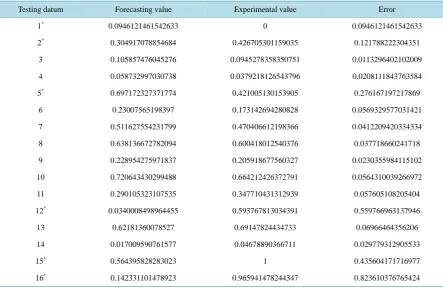
Table 6. The forecasting value with testing datum i, and the rest which exclude i are training data.

Testing datum Forecasting value Experimental value Error

1* _{0.0946121461542633 0 0.0946121461542633}

2* _{0.304917078854684 0.426705301159035 0.121788222304351}

3 0.105857476045276 0.0945278358350751 0.0113296402102009

4 0.058732997030738 0.0379218126543796 0.0208111843763584

5* _{0.697172327371774 0.421005130153905 0.276167197217869}

6 0.23007565198397 0.173142694280828 0.0569329577031421

7 0.511627554231799 0.470406612198366 0.0412209420334334

8 0.638136672782094 0.600418012540376 0.037718660241718

9 0.228954275971837 0.205918677560327 0.0230355984115102

10 0.720643430299488 0.664212426372791 0.0564310039266972

11 0.290105323107535 0.347710431312939 0.057605108205404

12* _{0.0340008498964455 0.593767813034391 0.559766963137946}

13 0.62181360078527 0.69147824434733 0.06966464356206

14 0.017009590761577 0.04678890366711 0.029779312905533

15* _{0.564395828283023 1 0.435604171716977}

16* 0.142331101478923 0.965941478244347 0.823610376765424

*

[image:11.595.89.533.418.707.2]

3,8,10

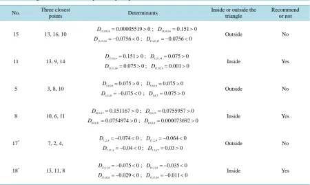
D and D_3,5,10 are opposite-sign, so, point 5 lies outside the triangle 3, 8, 10, it is not recommended to be a testing datum. Other cases are shown inTable 7, furthermore, if two new experiments No. 17 and 18 whose nondimensional parameters are respect (0.3, 0) and (0.7, 0.6) as shown inFigure 2 are conducted, according to the ES perceptron, No.18 is recommended to be a testing datum, while No.17 is not.

If a point lies outside the domain slightly, ES will found this, while SEH won’t. So, the domain determined by ES is smaller than SEH.

5. Conclusions

The important contribution of this paper is to answer such a question: why and how to distinguish the training data and testing data when uniform experiment design combined with nonlinear regression.

In this paper, two equivalent perceptrons which are the SEH perceptron and the ES perceptron are proposed to discover the topology boundary of the process parameter vectors and to distinguish training data and testing data. The distinguishing procedure is to determine if a testing datum lies inside the training datum domain. To give an application, experiments about laser cladding layer quality forecasting are conducted to prove if it is better that SEH or ES combines with SVR. The forecasting values of the testing data recommended by the two perceptrons are compared with their experimental values which are conducted based on uniform design. Results show that only the testing data recommended by the two perceptrons get a good forecasting by SVR, and the domain de-termined by ES is smaller than SEH.

So, the two perceptrons could guide experiments with process parameter data of complex topology structure. Further, not restricted to the experiment in this paper, the application could be extended over a wider field of experiments.

Acknowledgements

[image:12.595.88.539.437.706.2]

This work was supported by China Post-doctoral Foundation No. 2012M520572, Tianjin Municipal Education Commission Grant No.20120401, and Tianjin Municipal Science and Technology Commission Key Grant No. 14JCZDJC39500.

Table 7. Testing data recommended by the ES perceptron.

No. Three closest

points Determinants

Inside or outside the triangle

Recommend or not

15 13, 16, 10 13,10,16

0.00005519 0

D = > ; D15,10,16=0.151 0> 13,15,16 0.0756 0

D = − < ; D13,10,15= −0.0756<0

Outside No

11 13, 9, 14 D13,9,14=0.151 0> ; D11,9,14=0.075>0

13,11,14 0.075 0

D = > ; D13,9,11=0.001 0>

Inside Yes

5 3, 8, 10 3,8,10

0.075 0

D = > ; D5,8,10=0.075>0 3,5,10 0.075 0

D = − < ; D3,8,5=0.075>0

Outside No

8 10, 6, 11 D10,6,11=0.151167>0; D8,6,11=0.0755957>0

10,8,11 0.0754974 0

D = > ; D10,6,8=0.000073692>0

Inside Yes

17* _{7, 2, 4,} D7,2,4= −0.074<0; D17,2,4= −0.064<0 7,17,4 0.04 0

D = − < ; D7,2,17=0.03>0

Outside No

18* _{13, 11, 8} D13,11,8= −0.075<0; D18,11,8= −0.035<0 13,18,8 0.029 0

D = − < ; D13,11,18= −0.011 0<

Inside Yes

*

Conflict of Interests

None.

References

[1] Li, Y.W., Su, L., Zhang, X.Y., Huang, X.Y. and Zhai, H.L. (2011) Prediction of Association Constants of Cesium Chelates Based on Uniform Design Optimized Support Vector Machine. Chemometrics and Intelligent Laboratory Systems, 105, 106-113. http://dx.doi.org/10.1016/j.chemolab.2010.11.005

[2] Li, W.H., Liu, L.J. and Gong, W.G. (2011) Multi-Objective Uniform Design as a SVM Model Selection Tool for Face Recognition. Expert Systems with Applications, 38, 6689-6695. http://dx.doi.org/10.1016/j.eswa.2010.11.066

[3] Yu, X.L., Zheng, H.B., Yan, Q.S. and Li, W. (2011) A Least Square Support Vector Machine Approach Based on Uniform Design Method for Structural Reliability Analysis. Advanced Materials Research, 163-167, 3348-3353. http://dx.doi.org/10.4028/www.scientific.net/AMR.163-167.3348

[4] Zhang, G.Y. and Ge, H.H. (2012) Prediction of Xylanase Optimal Temperature by Support Vector Regression. Elec-tronic Journal of Biotechnology, 15. http://dx.doi.org/10.2225/vol15-issue1-fulltext-8

[5] Ni, L.J., Zhang, L.G., Tang, M.Y., Xue, Z.B., Zhang, X., Gu, X. and Huang, S.X. (2012) Discrimination of Adultera-tion Cow Milk by Improved v-Support Vector Machines and near Infrared Spectroscopy. 2012 8th International Con-ference on Natural Computation, Chongqing, 29-31 May 2012, 69-73. http://dx.doi.org/10.1109/ICNC.2012.6234508 [6] Yu, X.L. and Yan, Q.S. (2011) Reliability Analysis of Self-Anchored Suspension Bridge by Improved Response

Sur-face Method. Applied Mechanics and Materials, 90-93, 869-873. http://dx.doi.org/10.4028/www.scientific.net/AMM.90-93.869

[7] Xiang, C.S., Yuan, Z.M. and Zhou, Z.Y. (2011) Parameters Joint Optimization of Chaotic Time Series Prediction Model. Information and Control, 40, 673-679.

[8] Wang, Z.M., Tan, X.S., Yuan, Z.M. and Wu, Z.H. (2010) Parameters Optimization of SVM Based on Self-Calling SVR. Journal of System Simulation, 22, 376-378.

[9] Chuang, S.C. and Hung, Y.C. (2010) Uniform Design over General Input Domains with Applications to Target Region Estimation in Computer Experiments. Computational Statistics & Data Analysis, 54, 219-232.

http://dx.doi.org/10.1016/j.csda.2009.08.008

[10] Pan, J.-S., Hong, M.-Z., Zhou, Q.-F., Cai, J.-Y., Wang, H.-Z., Luo, L.-K., Yang, D.-Q., Dong, J., Shi, H.-X. and Ren, J.-L. (2009) Integrated Application of Uniform Design and Least-Squares Support Vector Machines to Transfection Optimization. BMC Biotechnology, 9, 52. http://dx.doi.org/10.1186/1472-6750-9-52

[11] Wang, X., Zhang, C., Li, P., Wang, K., Hu, Y., Zhang, P. and Liu, H.X. (2012) Modeling and Optimization of Joint Quality for Laser Transmission Joint of Thermoplastic Using an Artificial Neural Network and a Genetic Algorithm.

Optics and Lasers in Engineering, 50, 1522-1532. http://dx.doi.org/10.1016/j.optlaseng.2012.06.008

[12] Sun, Y.W. and Hao, M.Z. (2012) Statistical Analysis and Optimization of Process Parameters in Ti6Al4V Laser

Clad-ding Using Nd:YAG Laser. Optics and Lasers in Engineering, 50, 985-995. http://dx.doi.org/10.1016/j.optlaseng.2012.01.018

[13] Yang, D.X., Li, X.Y., He, D.Y., Nie, Z.R. and Huang, H. (2012) Optimization of Weld Bead Geometry in Laser Welding with Filler Wire Process Using Taguchi’s Approach. Optics & Laser Technology, 44, 2020-2025.

http://dx.doi.org/10.1016/j.optlastec.2012.03.033

[14] Beygi, H., Vafaeenezhad, H. and Sajjadi, S.A. (2012) Modeling the Electroless Nickel Deposition on Aluminum Na-noparticles. Applied Surface Science, 258, 7744-7750. http://dx.doi.org/10.1016/j.apsusc.2012.04.132

[15] Wang, Z.F. and Wang, H. (2012) Inflatable Wing Design Parameter Optimization Using Orthogonal Testing and Sup-port Vector Machines. Chinese Journal of Aeronautics, 25, 887-895.

http://dx.doi.org/10.1016/S1000-9361(11)60459-7

[16] Wang, Y. and Fang, K.T. (1981) About Uniform Distribution and Experimental Design: Number Theory Method.