Energy Efficient Coverage for Mobile Sensor Network
Richa Singh
Krishna Engineering College, Ghaziabad
ABSTRACT
Wireless sensor networks comprise the platform of a broad range of applications related to security system, surveillance, military, health care, and environmental monitoring. The sensor coverage problem has received lots of attention, being considerably driven by recent research in affordable and efficient integrated electronic devices. This problem is centered around a fundamental question: How well do the sensors observe the physical space? The coverage concept is subject to a wide range of interpretations due to a variety of sensors and their applications. Different coverage formulations have been proposed based on the pattern of sensor deployment and type of object to be covered as well as on other sensor network properties such as network connectivity and minimum energy consumption.
In this paper, we propose an energy efficient coverage algorithm to extend the sensor network lifetime while maintaining sensing coverage by sensor replacement mechanism. This sensor replacement mechanism manages fault repair in absence of location information. These algorithms keep a small number of active sensor nodes for less energy consumption.
Keywords – Coverage; Connectivity; Energy Efficiency; Node scheduling; Sensor networks and Reliability.
1.
INTRODUCTION
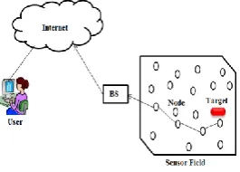
A wireless sensor network is collection of large number of sensor devices or motes called sensor nodes. These sensor nodes equipped with sensor unit, a transceiver unit, battery unit and programmable embedded processor. The sensor nodes are capable of sensing, data processing, and communicating with each other via radio transceivers [1]. They coordinate with each other to establish a network to remotely interact with the physical world, such as to monitor a geographical region or a set of targets spread across a geographical region, and to report sensed data to the monitoring center, which is connected to the base station. Wireless networks can be random or deterministic deployed in physical environments to collect information from an area of interest in a robust and autonomous manner. Sensor nodes organize into networks and collaborate to accomplish a larger sensing task. Architecture of sensor network is shown above in figure 1.
[image:1.595.121.254.647.742.2]
Figure 1: Architecture of WSN
A group of sensors node coordinating with neighboring sensor nodes can perform a much bigger applications effectively & efficiently. In wireless sensor networks, there are some important prerequisites [2]. They are:-
(a). Sufficient Sensing Coverage, (b). Sufficient Network Connectivity and, (c). Energy utilization.
Sensing is one of the prime responsibilities of a wireless sensor network. To operate efficiently, a sensor network must provide satisfactorily sensing coverage and also network connectivity. By satisfactorily sensor network connectivity, sensor devices can communicate for data fusion and reporting to base station (BS). Sensing coverage characterizes the monitoring standard set by a sensor network in a desired region of interest. The coverage requirement for a wireless sensor network depends on the types of applications and also on the number of faults that it can tolerate [3]. The coverage issue is to study and solve how to make sure that the coverage range meets the expected application requirements. The connectivity issue concentrates on how to ensure that all the active wireless sensor nodes are able to communicate with each other. According to coverage problem, objectives and applications, coverage scheme can be split into three types. They are area, point and barrier coverage [4].
In area coverage problem, a set of sensors is given and distributed over a geographical region to monitor a given area.
In point coverage problem, a set of sensors is given and distributed over a geographical region to monitor a set of points (or targets).
Barrier coverage sensors are deployed to detect the intruder as they enter into area covered by sensor. A Strong barrier has no gap or loose point from where the intruder can enter without detection
The sensing range of a sensor is typically model as disk in the 2D space or as a sphere in the 3D space, with the sensor located in the center. The communication range of a sensor is modeled in the same way. A sensor can monitor all targets that fall in its sensing range. The data sent by the sensor can be received by all sensors that fall in its communication range. A sensor’s transmission range is typically larger than its sensing range.
Stringent power supply of wireless sensor nodes is the most critical limitation, because those nodes are usually powered by batteries that may not be possible to be recharged or replaced after they are deployed in hostile or hazardous environments [5]. Sensor nodes are prone to be failure. The over-loading of working sensor nodes will cause easily exhausted and failed. In addition to possible hardware or software malfunctions, sensors may fail because of severe weather conditions or other hash physical environment in the sensor filed. It is therefore crucial to construct a fault-tolerant. In this paper, we have presented an algorithm which is fault tolerated i.e. area is monitored by at least one working sensor.
conditions monitoring, security surveillance in military and battle-fields, industrial diagnosis, gas leakage detection, wildlife habitat monitoring, under water applications, fire detection, object tracking, distant health care and even monitoring of other planets such as Mars.
In most of these applications the environment could be unfriendly; the replacement of these batteries /energy sources in nodes may not be possible once they are deployed. This will remain untouched for a long time without any battery replacement. So, the development of power-saving algorithm for the establishment of these sensor networks can prolong their lifetimes, which are very essential. Our main goals are:
Move the sensor node to the heal the coverage hole and controlling the expected density to avoid data transmission collisions, which may cause loss and intern for retransmission and intern indirectly reducing some problems like radio interference, congestion .
We need to account for certain constraints associated with the sensor network. In particular, minimizing energy consumption is a key requirement in the design of sensor network protocols and algorithms. Since the sensor nodes are equipped with small, often irreplaceable, batteries with limited power capacity, it is essential that the network be energy efficient in order to maximize the life span of the network. In addition to this, wireless sensor network design also demands other requirements such as fault tolerance, scalability, production costs, and reliability. It is therefore critical that the designer takes these factors into account when designing protocols and algorithms for wireless sensor networks.
The rest of the paper is organized as follows. In section 2 briefly introduces the related work, section 3 Problem Statement. Section 4 describes about proposed work, 5 describe the experimental results and section 6 is conclusion of proposed work.
2.
RELATED WORK
In this paper, we survey recent contributions addressing energy-efficient coverage problems in the,
Wireless sensor networks in which sensor nodes do not move once they are deployed. Sensors have omnidirectional antennae and can monitor a disk centered at the sensor's location, whose radius equals the sensing range.
An important problem receiving increased consideration recently is the sensor coverage problem, centered around a fundamental question: How well do the sensors observe the physical space? In some ways, it is one of the measurements of the quality of service (QoS) of sensor networks. The coverage concept is subject to a wide range of interpretations due to a variety of sensors and applications. Different coverage formulations have been proposed, based on the subject to be covered such as area versus discrete points, the sensor deployment mechanism such as random versus deterministic, and other wireless sensor network properties such network connectivity and minimum energy consumption. Another consideration is that the energy of sensor networks is scarce, and it is always inconvenient or even impossible to replenish the power. One solution is to leverage redundancy of deployment to save power, for in most cases, the density of sensor nodes is much higher than needed. Node scheduling is used to achieve this goal. A set of active working nodes is selected to work in a round and another
random set in another round, meanwhile a high degree of coverage is maintained. All the other non-selected nodes are turned off into the sleeping mode that needs very little energy. In this way, the overall consumed energy of the sensor network can be saved and the network lifetime prolonged.
Tian et al. in paper [6], presented a node-scheduling scheme, which can reduce system overall power consumption, therefore enhancing network system lifetime, by turning off some redundant sensor nodes. Their coverage-based off duty eligibility rule and back off-based node-scheduling algorithm ensures that the original sensing coverage is maintained after turning off redundant nodes. They implemented their algorithm in NS-2 as an extension of the LEACH protocol. Then they compared the energy consumption of LEACH with and without the extension and analyzed the effectiveness of their scheme in terms of energy saving. Simulation results proved that their scheme can preserve the system coverage to the maximum extent. In addition, after the node-scheduling protocol turns off some of the sensor nodes, certain redundancy is still guaranteed. Normally, this method requires good number of working sensors. Moreover, the authors address only the coverage issues without touching the network connectivity problem.
In [7], the author presented the problem to improve networks lifetime (in terms of rounds) while preserving both target coverage and connectivity. This not only gives satisfied quality of service (QoS) in sensors networks, but also presents more options to changes the design a power efficient sensor scheduling. They studied and presented the Connected Set Covers (CSC) problem, used to solve the connected target coverage problem. Later they proposed a Three Phase Iterative algorithm to solve the CSC problem named TPICSC. The algorithm does not put any condition on the wireless network configuration (for instance, the number or distribution of the target points) or on the wireless sensor nodes (number of sensors /sensing and transmission ranges). The author analyzed and showed that the proposed algorithm has polynomial time complexity in worst case. But it has a long runtime and therefore is not feasible for large scenarios.
In [8], author developed a Coverage Configuration Protocol (CCP) that results different degrees of sensing coverage and also maintain network connectivity. The authors propose that coverage can imply connectivity only when sensors‟ communication ranges are not less than twice of their sensing ranges (Rc ≥ 2Rs). Apart from that, they
showed that the desired network connectivity of boundary sensing nodes and interior nodes are equal to the degree of coverage and twice the degree of coverage, respectively. Each deployed tiny node runs the k-coverage eligibility algorithm to determine the targeting coverage of a sensor network by observing at how intersection points between sensors‟ sensing ranges are covered by their neighbors. For the case when Rc < 2Rs, Coverage Configuration Protocol does not guarantee network connectivity. But, the authors integrated CCP with SPAN [5] to provide sensing coverage and along with network communication connectivity.
or are destroyed. A sleeping node wakes up occasionally to probe its local neighborhood and starts working only if there is no working node within its probing range. Geometry knowledge is used to derive the relationship between probing range and redundancy. In this algorithm, desired redundancy can be obtained by choosing the corresponding probing range. However, this derivation is based on the assumption that all the nodes have exactly the same sensing range. It is hard to find a relationship between probing range and desired redundancy, if nodes have different sensing ranges. Furthermore, the probing-based off-duty eligibility rule cannot ensure the original sensing coverage and blind points may appear after turning off some nodes, which is verified in our experiment. In [10], an algorithm, called Geographical Adaptive Fidelity (GAF) was proposed, which uses geographic location information to divide the area into fixed square grids. Within each grid, it keeps only one node staying awake to forward packets. These three node-scheduling schemes turn off nodes from communication perspective without considering the system’s sensing coverage. In fact, in wireless sensor networks, the main role of each node is sensing. Unusual event could happen at any time at any place. Therefore, if we only turn off nodes, which are not participating in data forwarding, certain areas in the deploying area may become “blind points”. Important events may not be detected [9].
3.
PROBLEM STATEMENT
Wireless sensor network, the major problem is coverage and network connectivity. Hence, the research is being applied to retrieve an optimum number of sensor nodes such that it would minimize the cost, drop-off the energy use and also minimize the message control overhead [11]. Another major issue in sensor network is fault tolerance. As we know that sensor node is fragile and battery constrained, so it might be probable that the sensor node destroy or die when we want continuous monitoring. In such scenario we require that the sensor network must have fault tolerance characteristic. The most important constraint in sensor network is to maintain coverage and connectivity, where coverage and connectivity together work as notch of QoS in the sensor network. This performance metric tells us how well an area is observed or addressed by the sensor node and how perfect this sensed information is which accumulated by these sensor nodes. Problem to maintain coverage and connectivity is to locate the sensor node. Sensor node must neither be placed too tight to each other such that they compute or sense the same event nor too far to each other to elude the establishment of coverage holes.
4.
PROPOSED WORK
The primary objective of our algorithm is to heal the coverage hole by using mobile sensor node, and to maintain average density in the sensor field. After maintain the average density put the redundant node into sleep state for extending the network lifetime [12]. We proposed a four phase deployment algorithm. In the 1st phase we randomly deploy the sensor node in the sensor field. In the 2nd phase, we determine the coverage hole, size and identify the grid to be healed. In the phase 3rd, we move the mobile sensor node to the coverage hole target grid while minimizing the movement of sensor node. In 4th phase, from each grid one
sensor is in active state and rest of the sensor node in sleep state. This sleep wake scheduling is scheduled according to energy level of each the sensor node. This paper has been made the following assumptions:
(a) Each sensor has position information and has uniform sensing range.
(b) The sensor network is sufficiently dense.
(c) The communication radius of the sensor node is not less than double times of the sensing radius of sensor node.(Rc>=2Rs)
(d) Sensor network is homogenous network.
(e) Sensor nodes have locomotion competency with a sensible speed
(f) Cluster heads have higher processing competency, power, and storing ability than sensor motes so that the method can be supervised.
(g)Sensor nodes are structured as clusters and the cluster heads execute data aggregation before transmitting the accumulated data to the base station.
(h)The Sink is motionless and posed far off from the nodes.
(i) Sensors node are time-synchronized.
(j) Sensors are randomly distributed into a 2-D field. (k)The all sensors node communicates each other via
wireless links.
In WSN, continuous uncovered area is called Sensing Hole. A mobile sensor network can be considered as a collection of distributed sensor nodes, which are capable of sensing, moving, communicating within its allowable range. Mobility equipped sensors are utilized to replace the failure nodes from that target area to improve the overall coverage. Faulty sensors are described as low energy sensors. In our algorithm we use mobile sensor nodes. The main objective for using mobile sensor nodes is to heal coverage holes after the initial network deployment, such that the area coverage can be maximized while incurring the least moving cost. When designing a hole healing algorithm, the following issues need to be addressed.
1. How to decide the existence of a coverage hole and how to estimate the size of a hole?
2. What are the best target locations to relocate mobile nodes to repair coverage holes?
3. How to dispatch mobile nodes to the target locations while minimizing the moving and messaging cost?
Hole detection and hole size estimation
When an event happened and it is not sense by any sensor such a distance where an event occurred is larger than its sensing range, then there exists a coverage hole and the size of the hole is considered as proportional to the distance.
Destination selection
After deciding the existence of a coverage hole and its size, a mobile sensor node need to identify the target location where it has to heals.
any sensor within a grid cell, the side length of the grid cell should be S = Rs/√2. To ensure that any node within a cell
can directly communicate with any other node in its four adjacent cells, the transmission range of a node should be at least the diagonal of the rectangle constructed from two adjacent cells and hence S = Rs/√2. Therefore, the cell size
can be chosen as S=min {Rs/√2, Rs/√2}
4.1 Algorithm:
Step 1: Calculate the average of sensor field, i.e., number of sensor node / number of grid.
Step 2: Calculate the load of each grid i.e., number of node in each in each grid.
Step 3: Compare the load of each grid with an average value; if load of grid is less than average value then grid is in underload state. If load of grid is greater than average value then grid is in overload state and if the load of grid is equal to average value then grid is in neutral state.
Step 4: Construct three array overload, underload and neutral and the element of this array is grid number of overload, underload and neutral state respectively.
Step 5: Check the 1st element of underload array with 1st, 2nd and 3rd element of overload array.
(i) Calculate the number of node require to heal the coverage hole in 1st element of underload array i.e., Average value- Number of node in that grid. (ii) Move the sensor nodes from overload grid to an
underload grid according:-
1. If 1st element of an overload grid has sufficient number of sensor nodes require to heal the coverage hole in 1st underload grid and if its distance is less than the 2nd and 3rd element of an overload grid then move the sensor node from 1st element of overload grid to 1st element of underload grid else,
2. Move the number of sensor node from 2nd element of overload grid to 1st element of an
underload grid if it has sufficient number of sensor nodes and its distance is less than 1st and 3rd element.
3. Otherwise moves the number of sensor node from 3rd element of overload grid to underload grid if it’s have sufficient number of sensor and its distance is less than 1st and 2nd element of an overload grid.
Step 6: Delete the entry from underload array and overload array if it’s load is equal to neutral state i.e, the number of node in that grid is equal to average value.
Step 7: Repeat step 5 to 6 until the neutral array size comes to nXn or size of underload array comes to NIL.
Step 8: For each grid put one sensor into a WAKE state. Put that sensor into WAKE state whose energy level is greater than other sensor node.
This approach can be explained by an example. Node is
randomly deployed in sensor field. Initial node deployment is shown in figure 2, which is shown above.
[image:4.595.345.534.72.238.2]Sensor field is partitioned into small grid. In this example we have 72 sensor nodes and sensor field is partitioned into 36 grids. Now first we calculate the average i.e. number of sensor node to the number of grid.
Figure 2: Initial deployment
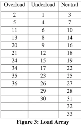
In our example average value is equal to 2 (72/36). Calculate the load of each grid. Now we determine the state of grid. Now we construct the overload, underload and neutral named array according the grid state. This array is show in figure 3 shown below:
Figure 3: Load Array
Now, 1st element of an underload array is compared with 1st, 2nd and 3rd element of overload array. In this comparison we checks the number of sensor nodes required to heal the coverage hole by underload array. In this example, an underload array 1st element is 1 which
means 1st grid, and it’s requiring 2 nodes to heal the coverage hole. Now this 1st element compares with the 1st
element of an overload array i.e. 2. This 2 means grid number 2, this grid number 2 has 2 extra nodes. It’s have sufficient number of nodes and its distance is less then 2nd and 3rd element i.e. grid number 5 and 7. After receiving this 2 sensor node, grid 1 become netural and its entry enter into netural array and deleted from underload array. Now underload 2nd element i.e grid 4 is compare with 1st and 2nd and 3rd element of overload array i.e. grid 5, grid 11 and grid 13 respectively. Here, grid 5 has only 1 extra nodes grid 11 has 3 extra nodes and grid 13 has only 1 node. Now we can see the grid 11 has sufficient number of nodes to heal the coverage hole and its distance is less then grid 5 and grid 13, so we move the sensor from grid 11 to grid 4. After getting this sensor nodes grid 4 become
31
2
32
2
33
2
34
3
35
3
36
4
25
2
26
0
27
2
28
2
29
1
30
1
19
2
20
4
21
6
22
2
23
1
24
3
13
3
14
2
15
1
16
2
17
0
18
2
7
2
8
1
9
0
10
2
11
5
12
1
1
0
2
4
3
2
4
1
5
3
6
0
Overload Underload Neutral
2 1 3
5 4 7
11 6 10
13 8 14
20 9 16
21 12 18
24 15 19
34 17 22
35 23 25
36 26 27
29 28
30 31
32 33
Grid No.
[image:4.595.359.502.313.532.2]netural and its entry is deleted from underlod array and its is made in neutral array. This is show in figure.
[image:5.595.99.243.107.353.2]
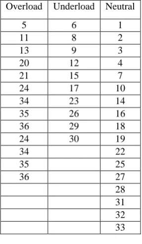
Figure 4: After 2nd round, Load Array
[image:5.595.336.505.626.741.2]Same procedure is repeated until netural array size become n X N ( in this example 72), or underload array become NIL. After all this step sensor nodes become netural is shown in figure 5.
Figure 5: Load Balance
After this load balancing, from each grid only one sensor node is in active state for a round. This is decides on the basis of the energy level. Those sensor nodes have high energy level as compare to other sensor nodes is put in into active state. After the round completed we again check the energy level and according to that energy level one of the senor node is put into the active state. This load balancing and sleep wake scheduling is continued till network lifetime. Now, if one of the sensor nodes dies then grid which have extra sensor node moves their senor to the location where sensor node died or where there is coverage hole. This algorithm minimize the move of the sensor node to reduce energy consumption
5.
EXPERIMENTAL RESULTS
The performance of the “Energy Efficient Coverage using Mobile Sensor Network” in the paper is evaluated
by simulation. We simulate the performance of energy efficient coverage scheme using MATLAB 7.10.0 in order to investigate coverage and connectivity, energy efficiency and network lifetime with LEACH and Sleep Wake scheduling scheme. We randomly deploy the sensor node on 70m X 70m sensor field area. The sink node is deploying at middle of sensor field. In our simulation analysis, we assume that the sensor node have mobility features.
The table 1 summarizes the simulation parameters used which shown above:
5.1 Energy Consumption Analysis
For energy calculation we use the first order radio model
[13]
. The equation used to calculate transmission cost and receiving costs for a 1-bit message and a distance d are respectively shown in figure 6.
Figure 6:First Order Radio Energy Model Overload Underload Neutral
5 6 1
11 8 2
13 9 3
20 12 4
21 15 7
24 17 10
34 23 14
35 26 16
36 29 18
24 30 19
34 22
35 25
36 27
28 31 32 33
31
2
32
2
33
2
34
2
35
2
36
2
25
2
26
2
27
2
28
2
29
2
30
2
19
2
20
2
21
2
22
2
23
2
24
2
13
2
14
2
15
2
16
2
17
2
18
2
7
2
8
2
9
2
10
2
11
2
12
2
1
2
2
2
3
2
4
2
5
2
6
2
Network (field) Size (L*W)
70 X 70m
Number of sensor nodes (N)
140
Location of the sink node
(35, 35)
Sensor nodes deployment
Random deployment
Data size 4000 bits
Data size 140
Mobility model Random waypoint model
Radio model First order radio model
Battery Initial capacity is presumed
to be fixed
Traffic model CBR traffic for periodic data generation
Sensing Range 10 m
Communication
Range 20 m
Grid size 10 m
Sensing Speed 1-20 m/s
Network Simulator Version
To transmit a 1-bit message a distance d, the radio expends:
Where, Eelec is the electronic energy which depends upon
issues such as the filtering, digital coding, and spreading of the signal. Emp is the amplifier energy. The Emp, Efs, and d2,
d4 depend on the bit error rate, the remoteness of the receiver. The do is a distance constant. When receiver
receives the message then its energy dissipation is
calculated by given formula:
We consider the energy consumed by sensor nodes is due to sensing and communication operation. Sensor nodes do not consume while it is in sleeping state. To evaluate energy efficiency of all the protocol, we compute the average energy use per round for all the protocol for 3000 rounds. The LEACH protocol has consumed 50 % (70 J) of average energy at 2100 round, where sleep wake protocol consumed average energy 21.5 % (30 J) at 2300 round. The average energy use for our proposed algorithm is very less as compared to LEACH, and sleep wake protocol energy i.e. till 2800 round it consumed up to 11 % (15 J) of average energy per round.
Figure 7. Comparison of Energy Efficiency
5.2 Coverage
Generally, coverage can be considered as the measure of quality of service of a sensor network. In this paper, coverage [14] is defined as the ratio of the union of areas (in square meters) covered by each active sensor node and the area (in square meters) of the entire ROI. Here, the covered area of each node is defined as the circular area within its sensing radius, Perfect detection of all interesting events in the covered area is assumed
C=Ui=1,…NAi/A
Where Ai is the area covered by the ith node; N is the total
number of active sensor nodes; A stands for the area of the ROI.
If a node is located well inside the ROI, its complete coverage area will lie within the ROI. In this case, the full area of that circle, i.e., πR2, is included in the covered
region. If a node is located near the boundary of the ROI, then only the part of the ROI covered by that node is included in the computation. Because of the areas covered by nodes that fall out of the ROI and the overlap of covered areas between nodes, one needs to use more nodes
than simply the ratio of and the area sensed by a single node.
The overall coverage of a sensor network is composed of the covered regions of each sensor node. Though the coverage of a sensor is expressed by a sensor model which is binary or stochastic, the overall coverage of a sensor network depends on the locations of the sensor nodes in the sensor field. The topology including the locations and spacing of sensor nodes determines the overall coverage of the network as well as the expected lifetime of the network.
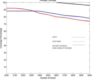
[image:6.595.101.260.361.491.2]For evaluating the coverage metric, we run all three schemes for 3000 rounds. Firstly we have seen result for 1000 rounds. In LEACH protocol, the average coverage for 1000 round is 92%, whereas for sleep wake scheduling protocol the average coverage for 1000 rounds is 88%.
Figure 8: Comparison of Average coverage for 1000 round
[image:6.595.361.509.585.713.2]In our proposed scheme, the average coverage for 1000 rounds is 100% which is more outstanding than other two schemes. We can say our proposed scheme provide full area coverage for long network lifetime. Comparison of all three schemes for 1000 round is shown in figure 8 above: Now, we compare all three scheme for last 1000 thousand round out of 3000 rounds. In LEACH protocol, the average coverage metric for last round is 74% whereas for sleep wake scheduling average coverage is 78%. For our energy efficient coverage scheme, average coverage is 97%. We could determine that the energy effective coverage for mobile network provide almost full coverage for entire network lifetime of sensor network. Where LEACH and sleep wake scheduling protocol does not put up all over coverage for entire network lifetime. The comparison of average coverage for last 1000 round i.e. from 2000 to 3000 round of all three algorithms is shown in figure 9.
5.3 Network lifetime
Network lifetime not measured by the time when first or last node dies but it is valued by the spell when network is available for providing facilities and operating correctly. Thus, network lifetime is firmly coupled with the sensor network performance. By running our algorithm, we conclude the lifetime of the network is raised up to 30%. As we view in figure 10, that LEACH protocol network lifetime is near 2200 round whereas our proposed algorithm network lifetime is approx. 2900 round.
[image:7.595.112.258.203.316.2]
Figure 10: Comparison of network lifetime
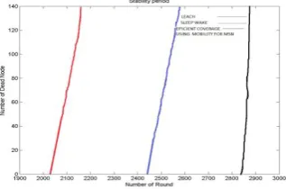
5.4 Stability
Stability period of WSN is the time interval for the first sensor node to die. Stability period is determined by efficient usage of available energy. In this figure 11, we can see that the stability period of LEACH protocol is 2030 round. Using sleep wake scheduling scheme in LEACH protocol, the stability period is increased up to 2450 round. And using our proposed algorithm the stability period reached to 2830 rounds. The stability period of our algorithm greater than LEACH protocol and Sleep wake scheduling protocol by 45% and 15% respectively.
Figure 11: Comparison, Stability of WSN
6.
CONCLUSION
Coverage with Connectivity is important factor for qualifying the QoS of wireless sensor network. The Sleep Wake scheduling mechanism used in our simulation is an energy-efficient as well as it sustain the coverage and connectivity of sensor network.
In this paper, we have presented the proposed “Energy
Efficient Coverage using Mobile Sensor Network”
algorithm for maintaining the number of sensor nodes in the sensor network and using the proper node scheduling i.e. ACTIVE and SLEEP. This proposed energy efficient coverage method for WSNs is compared with the normal
LEACH protocol and Sleep Wake protocol. Results from our simulations using MATLAB shows that the proposed protocol provides better performance in terms of energy efficiency and increasing level in lifetime of the wireless sensor networks.
7.
REFERENCES
[1] I.F. Akyildiz, W. Su, Y. Sankarasubrmaniam and E. Cayirci, Aug, 2002, pp 102-114, “A Survey on Sensor Networks”, IEEE Communication Magazine.
[2] D. G. Anand, H.G. Chandrakanth and M.N. Giriprasad, Volume 45– No.6, May 2012, “An Efficient Energy, Coverage and Connectivity Algorithm for Wireless Sensor Networks”, International Journal of Computer Applications
[3] M. Cardei, Jie Wu, 2006 “Energy-efficient Coverage Problems in Wireless Ad-hoc Sensor Networks”, Computer Communications, 29(4): 413-420.
[4] A. Gallais and J. Carle, “An Adaptive Localized Algorithm for Multiple Sensor Area Coverage”, in Proc.
of the 21st International Conference on Advanced
Networking and Applications
[5] Cardei, D. MacCallum, X. Cheng, M. Min, X. Jia, D.Y. Li, and D.-Z. Du, 2003, “Wireless Sensor Networks with
Energy Efficient Organization,” Journal of
Interconnection Networks, 213-229.
[6] D. Tian and N. D. Georganas, 2002, “A coverage-preserving node scheduling scheme for large wireless
sensor networks”, 1st ACM International Workshop on
Wireless Sensor Networks and Applications, Georgia, GA,
[7] Mohammad ali Jamali, Navid Bakhshivand, Mohammad Easmaeilpour, Davood Salami, “An Energy-Efficient Algorithm for connected target coverage problem in
wireless sensor networks”, 3rd
IEEE International
Conference Computer Science & Information
Technology (ICCSIT) on 9-11 July 2010,pp-249-254. [8] X.Wang, G.Xing, Y.Zhang, C.Lu, R.Pless and C.Gill,
2003, “Integrated Coverage and Connectivity
Configuration in Wireless Sensor Networks,” in ACM International Conference on Embedded Networked Sensor Systems, pp.28-39.
[9] F. Ye, G. Zhong, S. Lu, L. Zhang, Energy Efficient Robust Sensing Coverage in Large Sensor Networks, Technical Report.
[10] Y. Xu, J. Heidemann, D. Estrin, 2001 “Geography-informed Energy Conservation for Ad Hoc Routing, MOBICOM”.
[11] J. Joy Winston and B. Paramasivan, “A Survey on Connectivity Maintenance and Preserving Coverage for Wireless Sensor Networks”, International Journal of Research and Reviews in Wireless Sensor Networks, Vol. 1, No. 2, June 201.
[12] Khosrozadeh and H. Motameni, 2011 “Survey in Stable Coverage Guarded for Wireless Sensor Network”, American Journal of Scientific Research ISSN 1450-223X Issue 22, pp. 6-17.
[13] Heinzelman W. B., Chandrakasan A. P., and Balakrishnan H, 2002, “An Application-specific Protocol Architecture for Wireless Micro sensor Networks”, IEEE Trans. on Wireless Communications, pp.660-670. [14] A. Howard,M. J.Mataric, 2002, and G. S. Sukhatme, “An
[image:7.595.107.266.490.595.2]