Modeling of clay behaviour in pile loading test using one gravity small scale physical model

Modelling of Clay Behaviour in Pile Loading Test

using One-Gravity Small-Scale Physical Model

Sulaeman, A.

, Ling, F.N.L.

, & Sajiharjo, M.

1_{Faculty of Engineering Technology, Universiti Tun Hussein Onn Malaysia, Malaysia}

2_{Faculty of Civil and Environmental Eng., Universiti Tun Hussein Onn Malaysia, Malaysia}

a_{[email protected],} b_{[email protected],} c_{[email protected].}

Keywords: pile loading test; scaling factor; small scale modeling; critical state line clay.

Abstract. The observations and tests under small scale in 1-gravity condition are intended to obtain a comparative behavior of a model and prototype of geotechnical case by imposing the scaling relations. Simulations to represent a related structure, sub-soil and failure mechanism need to be prepared prior to do observations in this modeling. To simulate pile loading test (PLT) on clay, the following models of: clay, pile, driving simulation and procedure of PLT based on ASTM D4410 were set-up. The PLT in reduced scale environment was then followed by performing normal practice of full scale PLT in original clay site. Load settlement curves obtained from both “pile loading test” in small and full scale simulations showed closely good agreement. Further observation and investigation on simulation of pile loading test in clay revealed that modeling the following: clay sub-soil resulted in new properties of clay, em=ep+Ln(N) which reflects stress scaling factor, N, pile size and pile driving hammer need

scaling factor n and n3 respectively whereas PLT time needs time scaling factor, tp (n)0.5.

Introduction

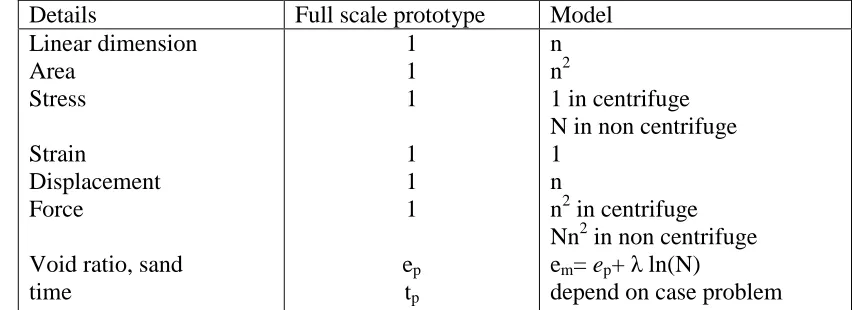
In a small scale physical modeling, there are some scaling factors (stress, force, weight, time, velocity, void ratio etc.) normally used to obtain the similarity behavior between model and prototype [2]. Different scaling factors are used in scaled modeling depending on a case problem to be observed. Table 1 shows the scaling factors normally implemented in 1-gravity and enhanced gravity environments.

Table 1: Scaling relations of the physical modeling approach 1-g and centrifuge environments.

Where: tp = time at prototype; n = geometric scale ratio

Details Full scale prototype Model

Linear dimension Area

Stress

Strain

Displacement Force

Void ratio, sand time

1 1 1

1 1 1

ep

tp

n n2

1 in centrifuge N in non centrifuge 1

n

n2 in centrifuge Nn2 in non centrifuge em= ep+ λ ln(N)

em = ep+ λ ln(N) (1)

where : em = void ratio model; ep = void ratio prototype; λ = critical state line (CSL) slope;

N= stress scale ratio

It has been mentioned that the em (Eqn. 1)is a void ratio in the model to simulate sand [3].

However, the usage of this formula to simulate cohesive soil is yet to be revealed.

In 1930’s the centrifugal devices was created, due to capital extensive in setting up this system, many attempts have been made to come up with a cheaper and effective system. The followings are some of them:

(i) NGI, 1981. Norwegian Geotechnical Institute in collaboration with Conoco Phillips [4] have

conducted scaled modeling using modified triaxial device to obtain the behaviour of single pile under cyclic and lateral load in an offshore structure;

(ii)Increased hydraulic gradient. The increased gradient method [5] scales the vertical stress

distribution by imposing a downward flow with a large, positive pressure gradient in the pore fluid in saturated soils used in the model.

(iii)Altae and Fellenius, 1994. In 1994, Altae and Fellenius reported that some examples of small scale test on bearing capacity of footings which have been published by many

researchers are unreliable due to the mistake in using similar void ratio (density) of model soil and prototype soil [6]. Then, they presented the new approach 1-g modeling in non-cohesive soil resulted in the use of void ratio of soil model should be different from prototype soil, em = ep +  Ln (N).

(iv) Frustrum Confining Vessel (FCV). A cone-shaped confining vessel for testing small scale

model piles was developed which controls the confining stress within the model soil mass by applying a vertical stress at the bottom of the soil mass [7]. The cone-shaped confining vessel is technically a frustum, the part of a cone left after the top has been cut off parallel to the base.

Testing Program

The following works program was intended to model all aspect in modeling of “PLT” which consists of laboratory and field loading test.

Laboratory Program. The following tests were done to the clay sample which was taken

from Research Centre for Soft Soils (RECESS), UTHM test site at 2-3 m depth. In order to prove that there was a relationship of scaling laws between model and prototype, “pile loading test” case was selected. To do so, the necessary aspects of modeling in small scale 1-g modeling were prepared i.e.: modeled soil (em), modeled pile, pile driving and loading mechanism of

PLT.

(i) Determination of modeled soil properties. Before properties of modeled soil was

determined, the engineering properties and critical state line (CSL) of clay soil at same location was previously measured by author [8]. Ten samples were taken from RECESS test site. Each sample was consolidated in triaxial until certain mean stress,

po = ( (2)

data from this test was plotted in e vs ln p and deviatoric stress vs strain to be analyzed to determine which curves coincide.

Once the analysis and calculation of soil model determined (em= 1.95), the original clay soil

was then modified to reach new void ratio and new unit weight indirectly. The modification was made by adding-up water into soil and mixed it up in such a way in order to produce void ratio em. Then the void ratio em in the modeling box was maintained unchanged to prevent from

extreme evaporation, the filled water tank was connected to this box.

(ii) Driving Simulation. To simulate the reinforced concrete pile of the size 15 cm in diameter

and length of 6 m, the aspect of scaling relation n = 10 was applied resulted in pile model having 1.5 cm width, length 60 cm and made from concrete mortar to represent similar roughness with real reinforced concrete pile.

In general, pile is driven by drop hammer. Certain hammer weight is dropped to reach a desired pile set. To simulate this, modeled pile was driven gradually by modeled hammer (actual hammer weight divided by scaling factor: n x n x n = n3 ; n represents scaling factors of length, width and height of hammer) to reach full length embedded. In this stage, actual hammer weight of 1 ton made normally by steel material was modeled by 1 kg pile hammer made by similar steel material.

(iii) Pile Loading Test (PLT) Simulation. Loading mechanism of pile loading test of Slow

Maintain (SM) [9] was utilized. This mechanism was then applied in small scale basis. Slow maintained loading test is normally performed on the measurement of load cell and displacement transducer in every 15 minutes. To determine the scaling factor “time” in pile loading test simulation, we need theoretical and mathematical approach which suits to this case problem.

The object in nature which can represent the pile motion during pile loading test can be simulated by equation of motion of the object [10] as follows:

In full scale (prototype):

MpAp+ CpAp+ KpAp = Fp (tp) (3)

In model (reduced scale ):

MmAm+ CmAm+ KmAm = Fm (tm) (4)

Manipulation to both expression resulted in

tm / tp= (Lm / Lp)0.5 ; (5)

Lm / Lp = n;

Hence :

tm / tp= (n)0.5 (6)

So, the rate of loading when pile moving down during loading test was controlled in such a way that it follows the scaling factor of time,

or

tm = 15(1/10)0.5 = 5 minutes. (8)

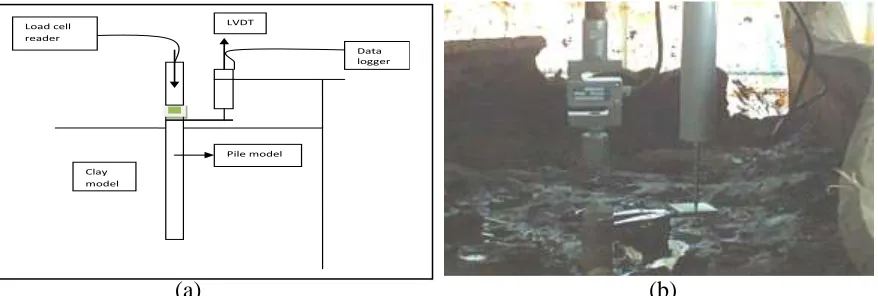
Other than that, the failure was also based on the following conditions: 10 % of pile width achieved 1.5 mm, no further resistance recorded in load cell and displacement recorded in the data logger were detected high, as shown in the Figure 1 (a) and (b) the PLT in small scale basis in schematic and being undertaken respectively.

(a) (b)

Figure 1: (a) Schematic PLT in small scale basis, (b) PLT in small scale basis was being undertaken

Field Test Program. The field test was intended to measure the real capacity of the piles. The

RC square pile, 150 x 150 mm, 6 m length was driven to field lab area.

(i) Driving the Piles. The pile was driven based on the normal practice of driving until all pile

length inserted. Waiting period of 30 days before commencement of full scale loading test was implemented to allow dissipation of pore water pressure in the vicinity of the pile. This was done to obtain true capacity of pile due to the conditions of soft clay and high ground water level at field lab Recess UTHM area.

(ii) Pile Loading Test. The concept of Kentledge system was adopted since this system

considered to be reliable. The procedure of test was based on the ASTM standard D 4410.

Results and Analysis

The followings are data results, analysis and verification of scaling factor of clay soil under PLT:

Engineering Properties. The engineering properties as shown in the Table 2 demonstrates

the very soft clay and high plasticity. Meanwhile, the Critical State Line (CSL) value, λ= 0.191 [8] had been investigated earlier by author.

Table 2: Engineering properties of RECESS soil

Depth (m)

Class Atterberg Limits Oedometer test Triaxial CU

2.0 – 3.0 CH MC = 57; LL= 68; PL = 27; PI = 41

Cv = 0.9 m2/year; Cc = 0.51

c= 7kPa ; Φ = 8° Data

logger Load cell

reader r

Clay model

To verify the correctness of CSL value, let refer to the expression of (Atkinson and Bransby, 1978) . Hence, Cc = 0.191 x 2.303 = 0.44. This number is not too far with actual site

condition of soft clay (Cc in the range of 0.40 to 0.55).

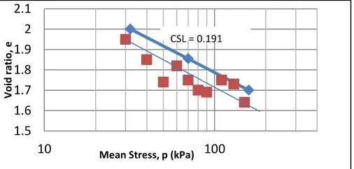
Lab Work. Lab work results to obtain similarity consist of scattered 10 data as a result of 10

samples subjected to different each initial mean stress. To comply with similarity, it is imperative to investigate which one of these scattered data is parallel to CSL. Figure 2 shows a result of plotted ten samples consolidated in triaxial and the Critical State Line of this clay soil. The similarity behavior of two samples would be found when

1) σ-ε curve was similar or the deviatoric stress was normalized by initial mean stress po also

coincide and

2) in e vs Ln p graph, the two data connected in one line is parallel with CSL of original soil [2].

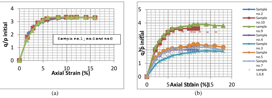
To follow this, all σ-ε of ten data were observed and the results was negative, instead when the curves were normalized by it’s po, it showed 3 curves of no.1 , 6 and 8 coincide.

By the guidance of the Figure 2, the following is the calculation of correlation between em and

ep. Let void ratio of soil model represented by e1 and void ratio of original clay prototype was e8

or e6 depending on how much N is planned.

Figure 2: Scattered mean stress vs void ratio

a) Sample 1 and 8

e1 = 1.95 ; e8 = 1.64 ; λ =0.191 ; em = ep +  Ln N ; 1.95 = 1.64 + 0.191 Ln N

Hence, N = 5 ; For verification, po8 = 150 kPa and po1 = 30 kPa , N also ratio of po8 to po1

b) Sample 1 and 6

e1 = 1.95 ; e6 = 1.82 ; λ =0.191 ; 1.95 = 1.82 + 0.191 Ln N ;

Hence, N = 2 this is in accordance with ratio of po6 = 60 kPa and po1 = 30 .

It is also noted that when sample 1, 6 and 8 are connected, it produces a line which is parallel to CSL. This is in conformity to the concept of similarity. Shown in the Figure 3a, the three normalized curves is identical as to compare with other curve in Figure 3b.

Thus, it can be concluded that stress scaling factor N resulted from modification of original soil into em in e – ln p environment can be used to simulate stress ratio in 1-g environment. In

enhanced gravity/centrifuge test, increased gravity is released to reach desired stress. However, stress level in 1-g model can be reached by modification an original prototype soil.

1.5 1.6 1.7 1.8 1.9 2 2.1

10 100

V

oi

d

rat

io,

e

Mean Stress, p (kPa)

(a) (b)

Figure 3: (a) Normalized deviatoric stress to initial mean stress of sample 1, 6 and 8 and (b) Normalized deviatoric stress to initial mean stress of all 10 samples

Small Scale Model. In the small scale basis, the data which was taken from instrumentations

was the raw data and should be converted by scaling factors. Using scaling factor for geometry n = 10, and N = 5 , Load F become Nxn2 = 5 x 102 = 500. It was noted that ultimate capacity of the pile was 21 kN as can be measured from converted L-S curve shown in Figure 4.

Full scale. In full scale pile loading test, all the readings was not necessarily converted. Shown in the Figure 4 the ultimate capacity was approximately 22 kN.

Figure 4: L-S curve from full scale loading test and Converted L-S curve from small scale

Although the ultimate capacity from small scale and full scale almost similar, there is a difference in the onset of failure. The first is reaching ultimate at 1.5 cm displacement whereas the latter failed at 2.2 cm. The slight difference of the curves shown in the Figure 3a and 3b is possibly due to other scaling factor which is not taken into account i.e.: friction/ roughness and stress history of soil. It is not well established to scale down the roughness, the roughness measurement needs special equipment as well as to produce scaled roughness of concrete surface. To obtain stress history similar between model and prototype is also another difficulty. It might be concluded that many scaling factors to be considered is likely to be more accurate. The result of Qu measured from PLT and small scale was around 21 kN. Although slightly

deviated, the amount of different was not significantly big and this result was encouraging. 0

1 2 3 4

0 5 10 15 20

q

/p

in

itial

Axial Strain (%)

0 1 2 3 4 5

0 5 10 15 20

q

/p

in

itial

Axial Strain (%)

Sample no.2 Sample no.10 sample no.9 Sample no.4 Sample no.3 Sample no.5 Sample no.7 sample 1,6,8 0 5 10 15 20 25

0 1 2 3 4 5 6 7 8 9 10

Load,

k

N

Pile settlement, cm

L-S curve of : small scale and full scale pile loading test

Full scale prototype

Conclusion

1. Simulation of geotechnical case in normal gravity to model geotechnical case problem need special attention to scaling factors.

2. The expression of em = ep +  Ln(N) can be applicable also for clay soil to modify original

soil into model soil.

3. The requirement of parallel with CSL means that the small scale model test should be performed in soil that is looser than prototype soil. This imposes boundaries on the scaling relations because; First, a model test cannot be performed in a soil looser than critical void ratio. Second, a model test must not be performed in a soil denser than prototype soil. Clay soil with too high of water content (high void ratio) tends to be more in liquid phase.

4. Complete scaling factors would result in a good accuracy, otherwise, less accuracy will be obtained.

Acknowledgement

This research was financially supported by Research Centre for Soft Soils (RECESS), UTHM. The authors are grateful to their supports and encouragements.

References

[1]Atkinson Bransby.(1978),“An introduction to critical state soil mechanics“McGrawhill (UK).

[2] D. M. Wood, C. Adam, and C. Taylor, Shaking table testing of geotechnical, International Journal of Physical Modelling in Geotechnics (IJPMJ) (2012).

[3] B.H. Fellenius, and A. Altae, Stress and settlement of footings in sand, Proceedings of ASCE, Geotechnical Special Publication, No.40 College Station, Texas (1994).

[4] K. Hange, and T. J. Kvalstad, Tension pile study, Norwegian Geotechnical Institute, (1981).

[5] A. Zelikson, Geotechnical model using the hydraulic gradient method. Geotechnique,Vol 19 (1996) pp.495-508.

[6] A. Altae, and B. H. Fellenius, Physical modelling in sand, Canadian Geotechnical Journal (1994).

[7] Stolle Horvart, Frustum confining vessel for testing model piles, Canadian Geotechnical Journal, 33 (1996) 499-504.

[8] A. Sulaeman, The use of lightweight concrete pile for foundations on soft soils, phD thesis, Universiti Tun Hussein Onn Malaysia (2010).

[9] ASTM D1143-81 Standard Test Method for Piles under Static Axial Compressive Load. American Society of Testing and Material (ASTM), USA, (Reapproved 1994) pp. 768-778.