Validation of PSIAC Model for Sediment Yields
Estimation in Ungauged Catchments of Tanzania
P. M. Ndomba
Department of Water Resources Engineering, University of Dar es Salaam, Dar es Salaam, Tanzania Email: [email protected]
Received May 23, 2013; revised June 27, 2013; accepted July 21, 2013
Copyright © 2013 P. M. Ndomba. This is an open access article distributed under the Creative Commons Attribution License, which permits unrestricted use, distribution, and reproduction in any medium, provided the original work is properly cited.
ABSTRACT
The main objective of this paper is to report on preliminary validation results of the newly applied sediment yields es-timation model in Tanzania, the Pacific Southwest Inter-Agency Committee (PSIAC). This is a follow-up research on the call to customize simple and/or multi-processes sediment yields estimation models such as PSIAC in the region. The PSIAC approach is based on a sediment yield classification scheme employing individual drainage basin characteristics: surface geology, soils, climate, runoff, topography, ground cover, land use, upland erosion, channel erosion, and sedi-ment transport. In this study, PSIAC model is built from readily available environsedi-mental variables sourced from Gov-ernment ministries/agencies and public domain global spatial data. The sediment classification exercise was verified with field observations. The set up model was then validated by 31 small dams’ siltation surveys and previous sedi-mentation study findings. PSIAC model performance for major part of central Tanzania was good during calibration (BIAS = 7.88%) and validation (BIAS = 18.12%). Another observation was that uncalibrated model performs fairly well, though performance improves with calibration. The extension of the uncalibrated PSIAC model to 3 selected large basins of Tanzania, with drainage areas size up to 223,000 km2, registered a satisfactory performance in one of them with fair performance in the rest. For large basins, the performance seems to correlate with general ground slope. The higher the slope, the better the performance. It is, however, not apparent from this study on the threshold drainage area and slope requirements for better performance of the model. Notwithstanding, the PSIAC model has improved previous sediment yields estimates based on simple regressive models. Finally, the paper proposes two main further research works: use of high resolution geospatial data and additional validation dams siltation data even beyond the central part of Tanzania, and carries out rigorous study on spatial scale model application limitations.
Keywords: Calibration; PSIAC Model; Sediment Yields; Tanzania; Validation
1. Introduction
Sediment yield in this paper refers to the amount of sediment exported by a catchment/basin over a period of time, which will eventually enter a lake, reservoir or pond located at the downstream limit of the catchment [1]. It represents total amount of fluvial sediment ex- ported by the catchment tributary to a measurement point (sampling station). Besides, sediment yield is a measure of the response of fluvial system to processes taking place in the drainage basin. Because much of eroded sediment is redeposited before it leaves a catchment, the sediment yield is always less than the upland erosion rates within that same catchment [1]. Available erosion- sediment yields estimation tools/models for a catchment vary greatly in complexity from simple regression rela- tionships to complex physics-based distributed simula-
tion models [2-4]. Modelling is one of the approaches for estimating catchment sediment yields [5].
management studies, researchers recommended for SWAT model improvements [6,8,9].
It should further be noted that most of the previous sediment yield estimates studies in Tanzania were catch- ment specific and resources (data, labour and time) in- tensive. Moreover, most erosion-sediment yields models such as SWAT are limited to simulating a specific ero- sion type, e.g., sheet. Hence modelling results in some studies could not be transferred easily to other hydrologic similar catchments [3,10,11]. In order to estimate catch- ment yield, researchers were forced to use uncertain fac- tors such as sediment delivery ratio [12]. The estimation tools used were either complex for operational and wider application or data intensive and could not be validated [13,14]. In any case, in Tanzania there is a very scanty knowledge about sedimentation and most of the catch- ments are poorly gauged [4,9,15]. Moreover, Tanzania like many other developing countries, has limited re- sources in terms of funding and human capital for de- veloping planning tools [4,11].
In a recent study by [4] sediment yields equations were developed for small catchments in Tanzania by regress- ing small dam sedimentation rates with catchment area. These were the only readily available data. The equations were developed for dry and moderate climate conditions. [4] admitted that the catchment size could not be directly related to erosion process, soil type, and land cover. Such limitations would render the developed sediment yield relationships useful only for preliminary planning pur- poses or as a rough check. Key limitations of [4]’s re- search findings include ill-defined study area as the wet climatic zone of Tanzania was not adequately repre- sented; and spatial lumping nature of model representa- tion using catchment area as the only independent vari- able. It was therefore recommended for future work to incorporate other parameters affecting sediment yield such as landuse, slope and soils.
In this study, a simple and more generic model, Pacific Southwest Inter-Agency Committee (PSIAC) [1,16,17], is used where sediment yield from all erosion types in an appropriate spatial scales is estimated. The PSIAC ap- proach is based on a sediment yield classification scheme employing individual drainage basin characteristics [16, 17]. The characteristics are surface geology, soils, cli- mate, runoff, topography, ground cover, land use, upland erosion, channel erosion and sediment transport. After evaluating individual factors for the whole catchment, the total index is calculated on the basis of summation of the scores of individual factors [16]. The scoring systems are employed to rank areas with specific environmental characteristics [18], thereby estimating their sediment yields.
In comparison with other approaches discussed before this framework demands less data and computational
resources. However, it was reiterated by [1] that the framework needs to be validated when applied in areas other than where it was developed. Despite the fact that PSIAC model has been tested elsewhere [19-21], to the best of author understanding, none is known on its per- formance on Tanzania ungauged catchments.
Therefore, the main objective of this paper is to report on preliminary validation results of the newly applied sediment yield estimation model, PSIAC, in Tanzania. This is a follow up research on the call to customize sim- ple and/or multi-processes sediment estimation models such as PSIAC in the region [4]. This research is linked to other initiatives in Tanzania such as those of sedimen- tology studies in 3 large basins of Tanzania, namely Lake Nyasa, Lake Tanganyika, and Pangani.
2. Material and Methods
2.1. Study Area Description
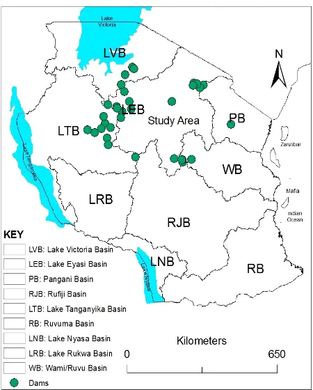
This study is about validating the performance of the multi-factors model, PSIAC, which on statistical grounds; it requires higher number of spatially distributed obser- vations than the model factors. The study considers ero- sion types mainly resulting from hydrospheric forces (i.e., rainfall, runoff and streamflows). Therefore, the study area was presupposed to cover various climatic regions. Following suit, the study area for model validation was dictated by the availability of small dams with siltation data and various climatic conditions representation in Tanzania (Figures 1-3).
Tanzania is located in eastern part of Africa continent and just South of the equator (Figure 1). It lies between
the area of the Great Lakes—Victoria (northern), Tan- ganyika (western) and Nyasa (South-West)—and bor- dered by the Indian Ocean on the East. Tanzania contains a total area of 945,087 km2 including 59,050 km2 of the inland water. Tanzania has a tropical climate with three (3) major climatic zones viz., wet, moderate and dry (Figure 2). Moderate climatic zone receives rainfall for 1
Figure 1. Location map of Tanzania.
Figure 2. Map showing climatic zones of Tanzania [26].
regime the March-May rains are referred to as the long rains or “Masika”, whereas the October-December rains
are generally known as short rains or “Vuli”. NB: The dots represent positions of the dams that were used in this study. Figure 3. Location map of the study area, central part of Tanzania with the spatial extent defined by small dams used in this study plus basins of Tanzania.
The study area, where majority of dam siltation data could be readily obtained, is the central part of Tanzania (Figure 3). It is mainly covered by a large plateau [22].
The plateau has a mean elevation of about 1100 masl, and consists of several precambrian terrains that have ex- perienced Cenozoic extension [22]. The southern half of this plateau is grassland within the eastern Miombo woodlands ecoregion. In the North the plateau is arable land and includes the national capital, Dodoma (Figure 1). Besides, the study area falls within the administrative
regions of Tabora, Singida, Shinyanga, Arusha and Do- doma.
2.2. Data and Data Analysis
2.2.1. Data Types and Sources
[image:3.595.62.282.313.548.2]validation include environmental variables, dam siltation and published sedimentation data as reported in [5,23,24]. Environmental variables such as geological and litholo- gical map with a scale of 1:250,000 of Tanzania [25] were used to extract surface geological features. The soil features were determined based on soil erodibility factor (USLE_K) from soil map of Africa. Climate was classi- fied based on [26] and mean annual rainfall map [27]. In SUA’s study the mean annual rainfall (mm/yr.) was es- timated based on available data from 1971 to 2000. Runoff factor was based and extracted from the Southern Africa average annual runoff map [28]. Topographic factor was determined based on average percentage of slope steepness. The average slope steepness was gener- ated from Digital Elevation Model (DEM) of 90 m reso- lution. The ground cover was evaluated based on frac- tional cover (FC). The land use was estimated based on economic activities on the land such as agriculture, graz- ing, deforestation, small scale mining, buildings or roads. The upland erosion and channel erosion information were obtained from the Global Assessment of Soil Deg- radation (GLASOD: [29]) and runoff maps.
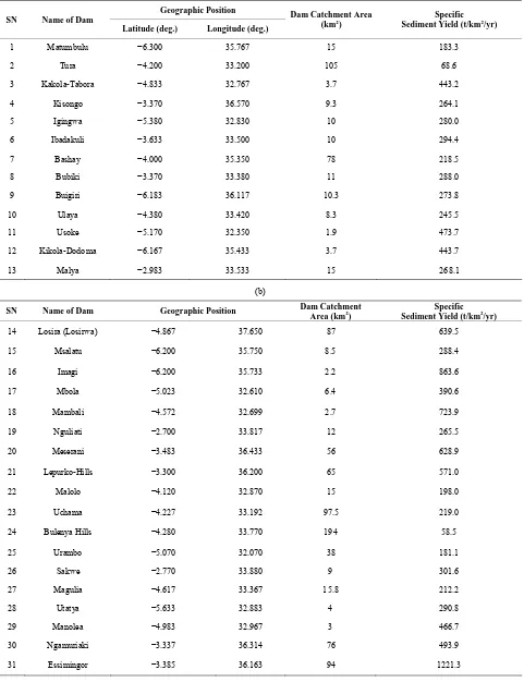
Data for fifty three (53) dams were collected with attributes including name of the dam, full supply level of the dam, capacity of the dam at full supply level, year of construction, accumulated sediment volume in the dam, year of dam survey, volumentric rate of sediment accu- mulation in the dam (sediment fill per year), geographic position, and catchment area. The dams were built for various purposes, including but not limited to irrigation, domestic water supply, livestock watering, flood control and fishing.
2.2.2. Data Analysis
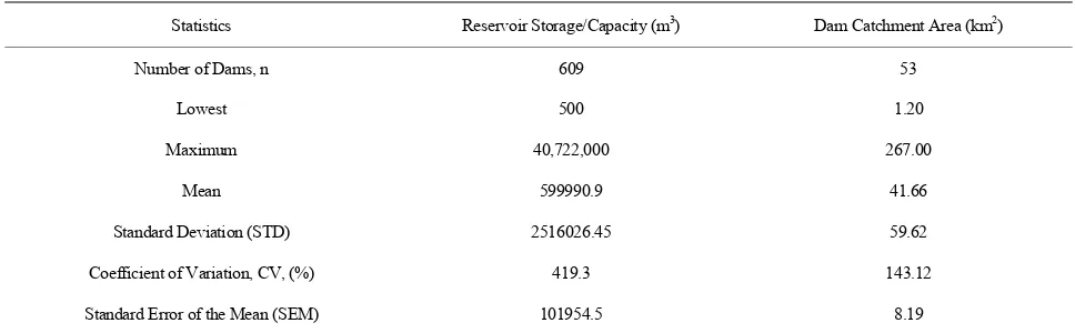
The statistics and physical characteristics of the selected water supply-irrigation small dams in Tanzania are pre-sented in Table 1. It should be noted, however, that
twenty two (22) dams were not included in the final analysis for two reasons: either their siltation data were considered outliers or dams’ geographical positions could
not be readily obtained.
A geographic position of the dam was crucial as it was used in this study to extract environmental variables from geospatial data/maps required for PSIAC model building. Therefore, only 31 dams with sediment yield data as presented in Table 2 were used for further analysis.
Specific sediment yield presented in the last column of
Table 2 was derived as the ratio of sediment yield to dam
catchment area.
As mentioned earlier under data types subsection the basic data for PSIAC model factor derivation were obtained from topographic maps, geological, soil, land use, ground cover, runoff, climate (mean annual rainfall), Normalized Difference Vegetation Index map (NDVI)- NOAA, and GLASOD maps. The data were used to generate spatial data layers and to evaluate the sediment factors based on PSIAC concept for the sediment model determination under GIS environment. Each river characteristic was scaled based on PSIAC sediment yield factor rating sheet [16,17]. All factors characterized by PSIAC model approach were described in a way of acquiring the PSIAC-Indices for each catchment. The PSIAC-Indices for the 31 dams selected were obtained through preparation, classification and assignment of weights according to PSIAC model building procedures. As illustrated in Table 3. Six (6) out of nine (9) river
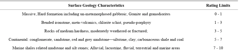
characteristics (surface geology, soil, climate, runoff, land use, and channel erosion) were acquired through interpolating the rating limits [17]. The interpolation was conducted based on corresponding characteristics of the spatial maps.
The surface geological map of Tanganyika was used to extract surface geological features. For instance, the volcanic and metamorphic rocks classified as massive and hard rocks were assigned a low rating limit. Mod- erate weathered and fractured rock, and ground surface of sand, silt, related with mudstones and siltstones were assigned a rating limit from 0 to 10 (Table 3).
[image:4.595.55.539.583.733.2]The soil features were determined based on soil
Table 1. Physical characteristics of the selected water supply-irrigation small dams in Tanzania.
Statistics Reservoir Storage/Capacity (m3) Dam Catchment Area (km2)
Number of Dams, n 609 53
Lowest 500 1.20
Maximum 40,722,000 267.00
Mean 599990.9 41.66
Standard Deviation (STD) 2516026.45 59.62
Coefficient of Variation, CV, (%) 419.3 143.12
Table 2. (a) Dams’ data used for model validation; (b) Dams’ data used for model validation.
(a)
Geographic Position
SN Name of Dam
Latitude (deg.) Longitude (deg.)
Dam Catchment Area (km2)
Specific Sediment Yield (t/km2/yr)
1 Matumbulu −6.300 35.767 15 183.3
2 Tura −4.200 33.200 105 68.6
3 Kakola-Tabora −4.833 32.767 3.7 443.2
4 Kisongo −3.370 36.570 9.3 264.1
5 Igingwa −5.380 32.830 10 280.0
6 Ibadakuli −3.633 33.500 10 294.4
7 Bashay −4.000 35.350 78 218.5
8 Bubiki −3.370 33.380 11 288.0
9 Buigiri −6.183 36.117 10.3 273.8
10 Ulaya −4.380 33.420 8.3 245.5
11 Usoke −5.170 32.350 1.9 473.7
12 Kikola-Dodoma −6.167 35.433 3.7 443.7
13 Malya −2.983 33.533 15 268.1
(b)
SN Name of Dam Geographic Position Dam Catchment
Area (km2)
Specific Sediment Yield (t/km2/yr)
14 Losira (Losirwa) −4.867 37.650 87 639.5
15 Msalatu −6.200 35.750 8.5 288.4
16 Imagi −6.200 35.733 2.2 863.6
17 Mbola −5.023 32.610 6.4 390.6
18 Mambali −4.572 32.699 2.7 723.9
19 Nguliati −2.700 33.817 12 265.5
20 Meserani −3.483 36.433 56 628.9
21 Lepurko-Hills −3.300 36.200 65 571.0
22 Malolo −4.120 32.870 15 198.0
23 Uchama −4.227 33.192 97.5 219.0
24 Bulenya Hills −4.280 33.770 194 58.5
25 Urambo −5.070 32.070 38 181.1
26 Sakwe −2.770 33.880 9 301.6
27 Magulia −4.617 33.367 15.8 212.2
28 Utatya −5.633 32.883 4 290.8
29 Manolea −4.983 32.967 3 466.7
30 Ngamuriaki −3.337 36.314 76 493.9
[image:5.595.59.540.114.740.2]Table 3. Surface geology factors and assigned rating limits.
Surface Geology Characteristics Rating Limits
Massive, Hard formation including un-metamorphosed gabbroic, Granite and granodiorites 0 - 1
Bended ironstone, meta-volcanics, chlorite schist, pseudo-porphyry 1 - 3
Rocks of medium hardness, moderately weathered or fractured; 3 - 5
Continental: conglomerate, sandstone, red and grey mudstone—siltstone, clay; carbonaceous shale and coal 5 - 7
Marine shales related mudstone and silt stones; Alluvial, lacustrine, fluvial, terrestrial and marine areas 7 - 10
erodibility factor (USLE_K) derived from FAO soil map of Africa. The map was acquired from global data sets available online. The study area soil erodibility factor values range from 0 to 0.426. The USLE_K for the soil rich in clays and organic materials defines a lower limit because such soils have low sediment generation potential. The soil characterized as silts, sand, and fine textures has higher USLE_K, hence, is defined as upper rating limit. The USLE_K was interpolated and resulted into the rating limits between 0 and 10.
Climate in this study is defined by range of mean annual rainfall amount. Rainfall is considered as the major contributor to soil erosion due to raindrop splashing impact and sediment entrainment [30]. The mean annual rainfall amount in mm/yr was estimated based on 30 years period of available data from 1971 to 2000. The mean annual rainfall ranging from 0 to 2400 mm/yr was assigned the rating limits between 0 and 10.
Based on mean annual runoff map for the study area, the extracted minimum and maximum mean annual runoff are 17 and 1250 mm/yr, respectively, with a mean of 531 mm/yr and CV of 62.4%. The corresponding rating limits are 0 and 10.
The rating limits for the remaining three PSIAC model environmental variables inputs (topography, ground cover, and upland erosion) were adopted from [17].
Topographic factor was determined based on average percentage of ground slope steepness. The Digital Elevation Model (DEM) of Africa acquired from global data sets that are available in USGS website was used to analyse an average percentage slope within the catch- ment.
Ground Cover factor was derived from vegetation, litter and rocks. The ground cover was evaluated based on fractional cover (FC) Equation, FC = 0.114 + 1.284 × NDVI, as adopted from [31]. The global datasets for NDVI map was obtained from [32]. The percentage of fractional cover was used to assign rating limits. The limits ranged from −10 to 10.
The land use was classified based on the status of soil degradation (GLASOD). The latter is expressed as the severity of the process. The severity is characterized by degree in which the soil is degraded and by relative
extent of degraded area within delineated physiographic unit. The rating limits of −10 and 10 correspond to severity levels of 0% and 100%, respectively.
The upland erosion was derived from both GLASOD and runoff maps. The severity of degradation is measured by the extent of rill and gully formation or mass movement. Potential upland erosion as represented/ measured by Severity was weighted/factored by runoff in order to infer upland erosion characteristics as presented in Table 4. It should be noted that both severity and
runoff were percentile classified.
Channel erosion was also derived from the GLASOD and annual runoff maps as for upland erosion factor. In this case a severity of sheet erosion was used. Potential channel erosion as represented/measured by Severity was weighted/ factored by runoff in order to infer channel physical characteristics.
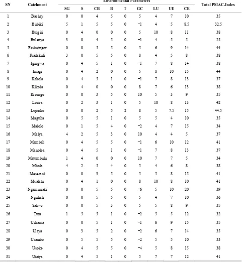
The total PSIAC index values are obtained by summation of evaluated individual factor indices for each catchment (Table 5). The PSIAC index combines the
PSIAC parameters as determinant factors to estimate specific sediment yield (SSY) for each catchment. Each catchment contained only one dam at the outlet. Classi- fication of sediment yield and rating under PSIAC model framework is presented in Table 6.
2.3. Development of a Sediment Yield Regression Model Based on PSIAC Concept
Considering scanty data from 31 dams with siltation data (Tables 2(a) and (b)), for validation purpose it was con-
sidered necessary to minimize the number of calibration parameters for the intended model. As recommended by [33] at least 10 to 20 times as many observations (cases, respondents) as variables, should be used for stable esti- mates of a regression line and replicability of results. In this case for PSIAC model with 9 determinant factors, a minimum of 90 observations would have been required for this analysis to arrive at meaningful confidence. In this context two types of regression model forms with a maximum of two model parameters were explored as candidates. These are straight line and power functions
Table 4. Upland erosion rating limits.
Upland Erosion Characteristics Percentage (%) Rating Limits
More than 50% of the area characterized by rill and gully or landslide erosion 50 - 30 25 - 13 About 25% of the area characterized by rill and gully or landslide erosion;
Wind erosion with deposition in stream channels 30 - 25 13 - 10
No apparent signs of erosion 25 - 0 10 - 0
Table 5. Factors indices and PSIAC-Index for 31 Dams.
Environmental Parameters SN Catchment
SG S CR R T GC LU UE CE
Total PSIAC-Index
1 Bashay 0 0 4 5 0 5 4 7 10 35
2 Bubiki 5 1 5 5 0 −1 4 5 8.5 32.5
3 Buigiri 0 4 0 0 0 5 10 8 11 38
4 Bulenya 3 0 4 5 0 −1 4 5 5 25
5 Essimingor 0 0 5 5 0 5 6 9 14 44
6 Ibadakuli 3 0 5 5 0 8 4 5 8 38
7 Igingwa 0 4 5 1 0 −1 7 8 14 38
8 Imagi 0 4 2 0 0 5 8 10 15 44
9 Kakola 0 4 5 1 0 −1 7 8 13 37
10 Kikola 0 4 0 0 0 8 7 6 13 38
11 Kisongo 0 0 3 5 0 10 5 3 9 35
12 Losira 0 2 3 1 0 5 10 8 13 42
13 Luperko 0 0 2 5 2 8 5 7.5 15 44.5
14 Magulia 0 5 5 1 0 5 5 4 10 35
15 Malolo 0 1 5 4 0 −2 4 7 15 34
16 Malya 4 2 5 3 0 10 4 4 5 37
17 Mambali 0 4 5 5 0 −1 6 10 12 41
18 Manolea 0 4 5 1 0 −1 7 8 13 37
19 Matumbulu 1 4 0 0 0 10 7 7 5 34
20 Mbola 4 2 5 4 0 5 4 6 8 38
21 Meserani 0 0 3 5 0 5 5 8 15 41
22 Msalatu 0 4 1 0 0 8 10 8 10 41
23 Ngamuriaki 0 0 5 5 0 −6 5 10 20 39
24 Nguliati 0 0 5 5 0 5 4 7 10 36
25 Sakwe 0 0 5 3 0 5 5 8 9 35
26 Tura 1 5 5 1 0 −2 5 5 12 32
27 Uchama 0 0 5 1 0 −1 6 9 15 35
28 Ulaya 0 3 5 2 0 −2 6 7 14 35
29 Urambo 0 5 5 5 0 −2 5 5 10 33
30 Usoke 0 4 5 5 0 −4 5 8 15 38
31 Utatya 0 4 5 1 0 5 7 7 12 41
[image:7.595.58.539.204.726.2]Table 6. Classification of sediment yield and rating as adopted from [16].
Class Rating Based PSIAC Index ( ) Sediment Yield (mm/yr)
1 >100 > 1.5
2 75 - 100 0.5 - 1.5
3 50 - 75 0.25 - 0.5
4 25 - 50 0.1 - 0.25
5 <25 <0.1
0 1 , 1, 2....,
i i i
Y X i n (1) where n is number of dam catchments, Xi is independent variable (PSIAC-Index or PSIAC based sediment yield estimate, PSIACSSY), Yi is dependent variable (measured sediment yield as estimated from dam siltation data, SSYdam and two parameters, β0 and β1), εi is an error term, and the subscript i indices a particular catchment.
i
Y Xi (2) where α and β are coefficient and exponent of the equation, respectively. The regression model for the linear function is done directly by using Yi and Xi values, while for the regression of the power function the logarithmic function is applied to the Equation (2) to obtain α and β coeffi- cients but both are regressed (Equation (3)). The powerful relationship is confirmed when its correlation is high on statistical grounds.
LogYiLog LogXi (3) The development of these equations was done under Excel spreadsheet environment using regression analysis and Analysis of variance (ANOVA) tool packs. In prin-cipal regression tool pack was first used to fit models to data, and then ANOVA was used to make sense of the fitted models, and to test hypotheses about the coeffi-cients.
2.4. Sediment Yield Model Performance Evaluation
The dams data sample size was divided into two sets for model calibration (70%) and validation (30%). Model validation involves running a model using input parame- ters measured or determined during the calibration proc- ess. Model validation exercise was meant to demonstrate that the fitted model is capable of making accurate esti- mation using an independent data set. The approach was considered as a superior and a more dependable method for measuring residuals.
Model evaluation techniques included at least one di- mensionless statistic Nash and Sutcliffe efficiency (NSE), one absolute error index statistics (RMSE), and other statistical information such as the standard deviation of
measured data. NSE could range from −∞ to 1. Essen- tially, the closer the model efficiency is to 1, the more accurate the model is. NSE values ≤ 0.5 are considered unsatisfactory [34], and NSE values ≤ 0 indicate the mean observed value is a better predictor than the pre- dicted values. Besides, NSE indicates how well the plot of observed versus predicted data fits the 1:1 line. Based on [35] the NSE coefficient is expressed in Equation (4). However, in the later section of this paper the NSE is presented in percent.
2 1 2 1NSE 1 i i i
i i
N m P N m m
(4)where N = number of dam catchments, mi= measured sediment yields (SSYdam), m = mean measured sediment yields, and Pi = predicted sediment yield.
Optimization of RMSE during model calibration may give a small error variance. The model was also evalu-ated through observation standard deviation ratio (RSR) and percent bias (PBIAS). RSR is the ratio of the RMSE and standard deviation of the measured data, as calcu-lated in Equation (5).
2 1 2 1 RMSE RSRSTDEVοbs
i i
i
i i
N m P N m m
(5)RSR ranges from 0 to a large positive value. Lower values indicate better model performance, with a value of 0 being optimal. It should be noted that in practice the optimal performance is rarely obtained. PBIAS measures the average tendency of the predicted data derived from the model to be larger or smaller than measured data. The optimal value of PBIAS is 0.0, with low-magnitude values indicating accurate model prediction/simulation. Positive values indicate model underestimation bias, and negative values indicate model overestimation bias. PBIAS was calculated using Equation (6).
PBIAS i i
i m P m
(6)based on [34] approach as follows: for PBIAS < 10% (very good); 10% - 15% (Good); 15% - 25% (satisfactory) and > 25% (unsatisfactory) for the calibration and valida-tion.
In some applications in this study, where validation data are limited, Relative Error measure, RE, was used to evaluate model performance. In such cases good per-formance is confirmed when RE in percent is less than 20%. This threshold is considered satisfactory for most of engineering practices.
Actual EstimatedRE % 100
Actual
(7)
3. Results and Discussions
3.1. Evaluated PSIAC Model Performance
As a first step of PSIAC model development, especially as it was applied for the first time in Tanzania, there was a need to investigate how the measured determinant fac-tors correlate with the measured sediment data. As de-picted in Figure 4 it was observed that measured
sedi-ment yields (SSYdam) correlate with PSIAC indices (PSIAC_Index) and PSIAC based sediment yield esti-mates (PSIAC_SSY) with coefficient of determination (r2) of 0.61 and 0.66, respectively. You will note that both PSIAC_index and PSIAC_SSY as independent variables and as presented into two separate horizontal axes (primary-lower and secondary-upper) share one vertical axis of measured sediment yields (SSYdam). Such presentation was intended to separate the two data sets for clarity purposes only. Otherwise, the data points would have clustered together. According to Student’s t-distribution with 29 degree of freedom, the read out table value at 5% level of significance, t0.05 is 2.045. As the computed t of 6.73 is greater than the table value, thus the correlation is considered significant [36]. As other researchers put it, typically r2 values greater than 0.5 are acceptable and warrant further analysis of the data [37].
This analysis suggests also that a strong correlation between measured and simulated sediment yield is con-firmed. Besides, the analysis allowed development of regressive sediment yield models using either PSIAC_Index or PSIAC_SSY as determinant factors, with the latter factor registering much stronger correla-tion. As explained in the methodology section above and as supported by correlation analysis, for further analysis, model calibration and validation, the estimated sediment yield (PSIAC_SSY) was used as determinant factor. Out of 31 dams 22 randomly selected were used for model calibration (Figure 5). Based on both qualitative and
quantitative analyses of scatter plot (Figure 5), the power
function was chosen as the best regression model for this
Figure 4. Scatter diagram of 31 data points between measured (SSYdam) and uncalibrated PSIAC based Sediment yields (PSIAC_SSY) and PSIAC indices (PSIAC_Index).
Figure 5. A scatter plot of measured and uncalibrated PSIAC based sediment yield data points plus fitted linear and power functions.
study. It can be seen from Figure 5 that the strength of
correlation increases substantially from linear (r2 = 0.64) to power (r2 = 0.73) functions.
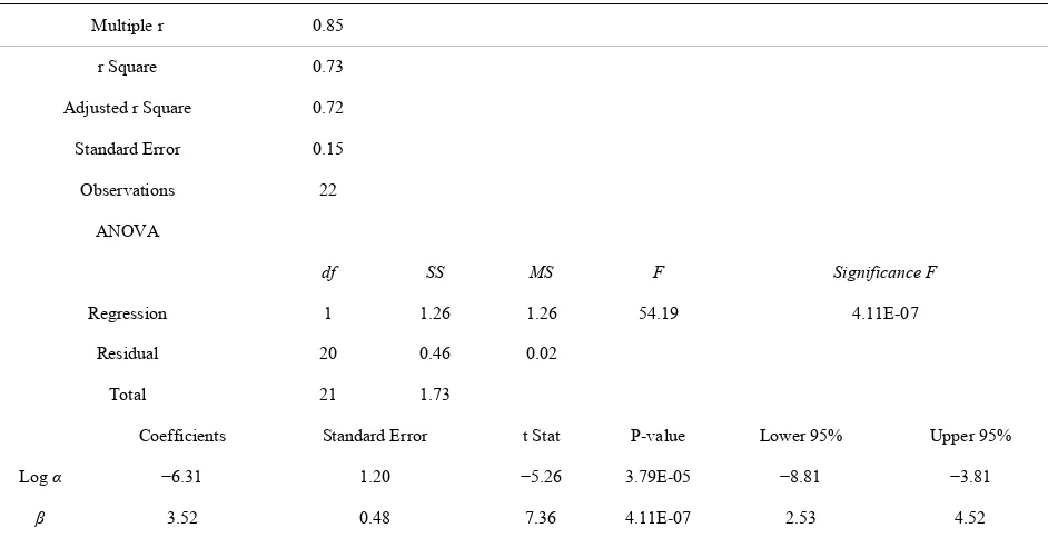
The regression output as presented in the Table 7 has
three main components: 1) Regression statistics table; 2) ANOVA table; and 3) Regression coefficients table. Therefore, regressively the coefficient (α = 4.91 × 10⁻⁷) and exponent (β = 3.52) of the power function were de-termined with the overall goodness-of-fit measure, r Square (r2) of 0.73. The resulting relationship is pre-sented in Equation (8).
3.527
SSY 4.91 10 PSIAC_SSY
[8]where, SSY and PSIAC_SSY are predicted and PSIAC based sediment yield, respectively, in t/km2/yr.
You will note from Figure 6 that the 45 degree line
(1:1 line) nearly bisects the 22 scatter points of calibrated model predicted SSY against measured/observed sedi- ment yield. Table 8 below further presents the perform-
Table 7. Regression statistics for power function.
Multiple r 0.85
r Square 0.73
Adjusted r Square 0.72
Standard Error 0.15
Observations 22
ANOVA
df SS MS F Significance F
Regression 1 1.26 1.26 54.19 4.11E-07
Residual 20 0.46 0.02
Total 21 1.73
Coefficients Standard Error t Stat P-value Lower 95% Upper 95%
Log α −6.31 1.20 −5.26 3.79E-05 −8.81 −3.81
[image:10.595.65.537.372.521.2]β 3.52 0.48 7.36 4.11E-07 2.53 4.52
Table 8. Evaluated PSIAC model performance.
Calibrated PSIAC Model Performance Indices
Calibration Validation
Uncalibrated PSIAC Model [4] Model*
No. of Data Points 22 9 31 22
r2 0.73 0.97 0.66 0.17
NSE (%) 59.90 68.50 19.70 −32.01
RMSE 0.46 0.50 0.56 0.59
RSR 0.63 0.56 0.89 1.15
PBIAS (%) 7.88 18.12 16.50 20
*Sediment yield estimates for moderate and dry climate of Tanzania [4].
tions), namely r2, NSE, RMSE, RSR and PBIAS. The model performance was reasonably good especially when evaluated against the PBIAS performance index.
The predicted catchments’ sediment yields based on the calibrated and validated model as presented in Equa- tion (8) vary from 61.76 t/km2/yr for Bulenya dam catch- ment to 772.82 t/km2/yr for Luperko dam catchment with an average of 358.29 t/km2/yr and coefficient of variation of 48.0%. Generally the calibrated model performance was better than that of uncalibrated, though they were equally good in terms of PBIAS performance index (Ta- ble 8). Comparison with previously developed model by
[4] in the same study area for moderate and dry climate indicates that the performance of the new model based on PSIAC concept has improved. These sediment yield es- timates are comparable to the ones reported in [38], who
[image:10.595.58.288.545.706.2]0 5 10 15 20 25 30 35 40 45 50 55 60 65 0 500 1000 1500 2000 2500 3000 3500
0 10 20 30 40 50 60 70 80 90 100
Gr o u n d sl o p e [% ] G ro und elev at io n [m a sl ]
Area coverage in (%)
Elevation_Nyasa Elevation_Tanganyika Slope_Nyasa Slope_Tanganyika 0 1000 2000 3000 4000 5000 6000
0 20 40 60 80 100
Area (%) G r o u nd E lev at ion [m as l] 0 5 10 15 20 25 30 35 40 45 50 G r oun d s lope [ % ]
Ground elevation Ground Slope
[image:11.595.64.535.86.279.2](a) (b)
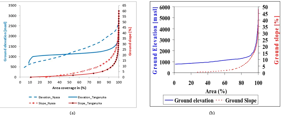
Figure 7. Distribution of ground elevation and slope with respect to area coverage in the 3 basins: Lake Nyasa, Lake Tanganyika and Pangani upstream of Nyumba Ya Mungu dam. (a) Lake Nyasa and Lake Tanganyika; (b) Pangani upstream of Nyumba Ya Mungu dam [5].
estimated sediment yields of 260 - 900 t/km2/yr or 2.6 - 9 t/ha/yr. as averages for the longest periods of available records. The principal methods employed include field surveying and air photo interpretation.
3.2. Extension of PSIAC Application to 3 Selected Large Basins of Tanzania
As there were no readily available small dams siltation data in other regions, other than the central part of Tan-zania, validation was made between uncalibrated PSIAC model sediment yields estimate and available published or report on sedimentation rates [5,23,24] and catchment sediment yield rates [39]. In this exercise, PSIAC model used spot based field observations data to estimate sedi-ment yield in three basins of Tanzania, viz., Lake Nyasa, Lake Tanganyika, and Pangani. It should be recalled that the performance of uncalibrated model in central part of Tanzania is presented in Table 8. Furthermore, as it was
not possible to compare directly between the spot level and the regional based published sediment yields by [39], thus statistics such as mean and range were used instead (Table 9).
The mean value of 5.064 t/ha/yr or 506.4 t/km2/yr, for Lake Nyasa basin is enclosed in the range 5 to 7.5 t/ha/yr. or 500 to 750 t/km2/yr. (
Table 9). with some degree of
confidence. Further validation of computed sediment yield results was done with respect to the observed Lake Nyasa sedimentation rate data as reported in [23]. Given the total area of 165,109 km2 for Lake Nyasa basin (33,457 km2 of water surface and 131,652 km2 of land area), the observed Lake Nyasa sediment deposition rate (66,914,000 t/yr) was determined as the product of lake area (33,457 km2) and sedimentation rate (1mm/yr or 2000 t/km2/yr) (
Table 10). Simulated sediment yield rate
of 54185850.31 t/yr from PSIAC approach is given by the product of Lake Nyasa basin on Tanzania side sediment yield rate (16,105,280 t/yr.) and total Lake Nyasa basin land area (131,652 km2) divided by Lake Nyasa basin on Tanzania side land area (39,130 km2). The Relative Error in percent, RE, of the estimate as computed using Equa- tion (7) is therefore equal to 19%. As the RE is below 20%, the performance of the model in Lake Nyasa basin is acceptable for most technical practical problems.
You will also note that the mean sediment load of 6.5 t/ha/yr. or 650 t/km2/yr. for Lake Tanganyika basin is enclosed in the range 5 to 7.5 t/ha/yr. or 500 to 750 t/km2/yr. with some degree of confidence (
Table 9). The
sediment yield for the entire drainage basin using PSIAC model (84,773,586 t/yr.) was computed as the product of Lake Tanganyika basin on Tanzania side sediment yield rate (57,402,746 t/yr.) and total drainage area of Lake Tanganyika basin land area (223,000 km2) divided by land area of Lake Tanganyika basin on Tanzania side (151,000 km2).
The computed sediment yield results were compared with observed Lake Tanganyika sediment deposition rate data as reported in [24]. Lake Tanganyika sediment deposition rate estimated based on a sample of 7 variates published in [24] varies from 0.085 (offshore) to 1.2 mm/yr. (near shore). Based on the published data, this study, on statistical grounds, has computed an average sedimentation rate of 0.32 mm/yr. with confidence limits between 0.031 and 0.61 at 5% level of significance. The observed sedimentation rate (20,864,000 ± 18,908,000 t/yr.) was estimated as the product of lake area (32,600 km2) and sediment deposition rate (0.32 ± 0.29 mm/yr or 640 ± 580 t/km2/yr) (
Table 10). Therefore, for the case of
Table 9. Validation of computed PSIAC model sediment yield rates with published data by [39].
Lake Nyasa Basin Lake Tanganyika Basin Pangani Basin
Statistics Calibrated
PSIAC (t/ha/yr)
Published Data (t/ha/yr)
Calibrated PSIAC (t/ha/yr)
Published data(t/ha/yr)
Calibrated PSIAC (t/ha/yr)
Published Data (t/ha/yr)
Mean 5.064 5 - 7.5 6.5 5 - 7.5 5.05 2.5 - 5
Sample Variance 3.605 - 8.580 - 9.918 -
Confidence Level (95.0%) 0.767 - 2.095 - 2.633 -
Standard Deviation 1.899 - 2.929 - 3.149 -
Standard Error 0.372 - 0.926 - 1.113 -
[image:12.595.55.546.102.242.2]Field Points 26 - 10 - 8 -
Table 10. Validation of computed PSIAC model sediment yield rates with published sedimentation rates by [5,23,24].
Lake Nyasa Basin Lake Tanganyika Basin Lake NYM in Pangani Basin
UnCalibrated
PSIAC Published Data
UnCalibrated
PSIAC Published data
UnCalibrated PSIAC
Published Data
Drainage Area (km2) 131,652 223,000 12,000
Lake Area (km2) 33,457 32,600 168
Percent (%) of Ground Area with Slope
Less than 3% (Figure 7) 54 74 73
Sedimentation Rate (mm/yr) 1 0.32 ± 0.29 Not determined
Sedimentation Rate (Mt/yr) 54.20 66.90 84.80 20.86 ± 18.91 5.99 0.411
Relative Error (%) 19 (<20) >20 >20
greater than 20%.
As presented in Table 9 the estimated mean sediment
yield rate for Pangani basin is 5.05 t/ha/yr. or 505 t/km2/yr. with a standard deviation of 3.15 t/ha/yr. or 315 t/km2/yr. You will note that it is enclosed within a range of 2.5 to 0.5 t/ha/yr. or 250 to 500 t/km2/yr. as published by [39]with some degree of confidence. It is worth not- ing that the mean annual sedimentation rate of 411,000 t/yr. at Nyumba Ya Mungu reservoir as reported in [5] is much less than the total sediment yield of 5.99 Million t/yr. as computed by PSIAC model for the 12,000 km2 NYM dam catchment area. Again, for the case of Pan-gani basin, the computed RE is greater than 20%.
The foregoing discussions suggest that the PSIAC model did not perform well in terms of estimating fur- thermost downstream outlets in 2 large study basins. In- dependent analysis as supported by Figure 7 suggests
that basin terrain characteristics might explain somewhat to the performance of the PSIAC model. For instance, one would note that about three-quarters of the Lake Tanganyika and Pangani upstream of Nyumba Ya Mungu dam basins are relatively flat with general ground slope of less than 3% (Table 10 and Figure 7). That is to
say, few meters increase in the ground height results into larger gain in area coverage. In the same basins, Figure 7
also depicts that about less than 20% of the area may be
[image:12.595.65.541.269.414.2]In all these analyses, for the three large basins, it is considered by the author that the larger the validation sample size the better the results. PSIAC approach was considered giving meaningful estimates for our region, especially in small catchments and large basins with mild slope such as Lake Nyasa basin. However, the author would like to acknowledge a number of uncertainties in this study. For instance, error due to digitization and georeferencing of the scanned maps for runoff, rainfall, and surface geology were assumed minimal. The spatial grid size of 0.020 degrees used determines the resolution at which the data were captured/obtained from the digi- tized maps and could have affected the results. Accumu-lation of error might have also resulted from the conver- sion of input data presented in vector to vector form and/or raster formats processing. Besides, the author would like to note that the sedimentation rates as deter- mined by previous studies [5,23,24] may have some de- gree of uncertainty. As reported in literature, all tech- niques for estimating reservoir volume incorporate errors [1] and may range from about ±10% to 30%. Therefore, the rates computed above were considered allowable as it is within the uncertainty range of Lake or sediment vol- ume estimates. However, for the case of Lake Tangany- ika the error could be higher as sedimentation rate data collected were localized in the central part of the lake, near Kalya horst. So the data are spatially ill-representa- tive as compared to data collected for Lake Nyasa by [23]. In particular, [24] admitted that certain limitations might arise when evaluating base level dynamics exclu- sively from core data. It should also be noted that the sediment yield estimates from Tanzania side of the ba- sins for the cases of Nyasa and Tanganyika were trans- ferred to the entire basin using specific sediment yield concept. In the latter approach, linearity was assumed. That is to say sediment yield contribution from all catchments around the lakes was assumed to be spatially constant.
4. Conclusions and Recommendations
The calibrated model was considered “good” (NSE = 60% and RSR = 0.63), and coefficient of correlation (r) of 0.85 for set of data used for model fitting/calibration. PBIAS values were relatively low and considered “very good” for specific sediment yield prediction, ranging from 7.88% to 18.2%. Besides, the performance of the uncalibrated model was equally good. These results demonstrate that PSIAC model can effectively estimate specific sediment yields in ungauged small catchments of Tanzania. The model might equally be extended to large basins with mild ground slopes. Thus, it can be a useful tool for evaluating potential sediment impacts within the study area to examine specific sediment yields.
The following specific recommendations are made
from the experience gained through this study:
1) Because of the simplicity of the implemented empiri- cal sediment model, Pacific Southwest Inter-Agency Committee (PSIAC), the present study estimated the model parameter indices on a qualitative basis. It is therefore recommended for future research to use a modified PSIAC model in order to estimate the pa- rameters indices objectively. It was not possible dur- ing this study to apply it due to resources limitations in terms of spatial data requirements, time and per- sonnel needed to estimate all PSIAC parameters using yet another model known as Bureau Land Manage- ment model.
2) Most of the dams data used, though few for model calibration and validation, were concentrated in the central part of Tanzania, hence further studies should use more data even beyond the central part of Tanza- nia.
3) It should be recalled that previous researchers else- where have indicated that this model performs better in small catchments with drainage areas size ranging between 0.05 and 86 km2. With spatial scale model application limitation, though indirectly investigated in this study with good performance in one of the 3 large basins of Tanzania, it is recommended to carry out rigorous study in future for the same purpose.
5. Acknowledgements
This work is part of the outputs of consultancy service in which the author as sedimentologist in a multidisplinary team charged by Ministry of Water with the responsibil- ity of preparing an integrated Water Resources manage- ment and development plans for 3 basins in Tanzania, namely, Lake Nyasa, Lake Tanganyika and Pangani. I also appreciate the assistance rendered to me by my postgraduate and undergraduate students, viz. Mdee, O., Sechu, G., and Hamisi, A., in carrying out some geospa- tial data analysis. The paper was critically reviewed by Prof. Mtalo, F.W. and Dr. Kahimba, F. of University of Dar es Salaam and Sokoine University of Agriculture, respectively. Some recent data and information on small dams in Tanzania were provided by Ministry of Water senior staff, Dr. George Lugomela, the Assistant director department of Water resources and Mr. Nkuba, the head of dam safety unit. Finally, I’m indebted to the Director- ate of Research of University of Dar es Salaam for cov- ering paper preparation cost and publication fees.
REFERENCES
[1] G. L. Morris and J. Fan, “Reservoir Sedimentation Handbook,” McGraw-Hill Book Co., New York, 1998. [2] R. J. Garde and K. G. Ranga Raju, “Mechanics of Sedi-
Third Edition, New Age International (P) Limited, Pub- lishers, New Delhi, 2000, 5p.
[3] P. M. Ndomba, “Modeling of Sedimentation Upstream of Nyumba ya Mungu Reservoir in Pangani River Basin,” Nile Basin Water Science and Engineering, Vol. 3, No. 2, 2010, pp. 25-38.
[4] P. M. Ndomba, “Developing Sediment Yield Equations for Small Catchments in Tanzania,” In: D. Chen, Ed., Advances in Data, Methods, Models and Their Applica- tions in Geoscience, InTech, China, 2011, pp. 241-260. www.intechopen.com
[5] P. M. Ndomba, “Modelling of Erosion Processes and Reservoir Sedimentation Upstream of Nyumba Ya Mungu Reservoir in the Pangani River Basin,” Ph.D. Thesis, Uni- versity of Dar es Salaam, Dar es Salaam, 2007.
[6] P. M. Ndomba and A. van Griensven, “Suitability of SWAT model in sediment yields modelling in the Eastern Africa,” In D. Chen, Ed., Advances in Data, Methods, Models and Their Applications in Geoscience, InTech, China, 2011, pp. 261-284. www.intechopen.com
[7] J. G. Arnold, J. R. Williams and D. R. Maidment, “Con- tinuous-Time Water and Sediment-Routing Model for Large Basins,” Journal of Hydraulic Engineering, Vol. 121, No. 2, 1995, pp. 171-183.
doi:10.1061/(ASCE)0733-9429(1995)121:2(171)
[8] A. van Griensven, P. Ndomba, S. Yalew and F. Kilonzo, “Critical Review of the Application of SWAT in the Up- per Nile Basin Countries,” Hydrology and Earth System Sciences, Vol. 16, No. 9, 2012, pp. 3371-3381.
www.hydrol-earth-syst-sci.net/16/3371/2012/doi:10.5194 /hess-16-3371-2012
doi:10.5194/hess-16-3371-2012
[9] P. M. Ndomba, F. W. Mtalo and A. Killingtveit, “Model in Sediment Yield Modelling for Ungauged Catchments: A Case of Simiyu Subcatchment,” EAWAG-Zurich, Zu- rich, 2005, pp. 61-69. www.brc.tamus.edu/swat
[10] M. K. Mulengera and R. W. Payton, “Estimating the USLE-Soil Erodibility Factor in Developing Tropical Countries,” Tropical Agriculture, Vol. 76, No. 1, 1999, pp. 17-22.
[11] M. K. Mulengera, “Sediment Yield Predictionin Tanzania: Case Study of Dodoma District Catchments,” Tanzania Journal of Engineering and Technology (TJET), Vol. 2, No. 1, 2008, pp. 63-71.
[12] P. M. Ndomba, F. W. Mtalo and A. Killingtveit, “Esti- mating Gully Erosion Contribution to Large Catchment Sediment Yield Rate in Tanzania,” Journal of Physics and Chemistry of the Earth, Vol. 34, 2009, pp. 741-748. www.elsevier.com/locate/pce
[13] P. M. Ndomba, F. W. Mtalo and A. Killingtveit, “A Guided SWAT Model Application on Sediment Yield Modeling in Pangani River Basin: Lessons Learnt,” Jour- nal of Urban and Environmental Engineering, Vol. 2, No. 2, 2008, pp. 53-62. doi:10.4090/juee.2008.v2n2.053062 [14] P. Lawrence, A. Cascio, O. Goldsmith and C. L. Abott,
“Sedimentation in Small Dams-Development of a Catch-ment Characterization and SediCatch-ment Yield Prediction Procedure,” Department for International Development (DFID) Project R7391 HR Project MDSO533 by HR,
Department for International Development (DFID), Wal- lingford, 2004.
[15] P. Z. Yanda, “Temporal and Spatial Variations of Soil Degradation in Mwisanga Catchment, Kondoa, Tanzania,” Ph.D. Dissertation, Stockholm University, Stockholm, 1995, 136p.
[16] PSIAC, Pasific Southwest InterAgency Committee, “Fac- tors Affecting Sediment Yield in the Pasific Southwest Area and Selection and Evaluation of Measures for Re- duction of Erosion and Sediment Yield,” Report No. HY 12, Water Management Subcommitte on ASCE, Reston, 1998.
[17] RCD, Resource Conservation District, “PSIAC Model: Sediment Yields in Sub-watersheds of the Petaluma River,” Resource Conservation District, Petaluma, 1998. [18] J. V. Vogt, R. Colombo and F. Bertolo, “Driving Drainage
Networks and Catchment Boundering. A New Method- ology Combining Digital Elevation Data and Environ- mental Characteristics,” Geomorphology, Vol. 53, No. 3-4, 2003, pp. 281-298.
doi:10.1016/S0169-555X(02)00319-7
[19] P. Bazzoffi, G. Baldassarre and S. Vacca, “Validation of PSIAC Model for Automatic Assessment of Resservoir Sedimentation,” In: M. Albertson, Ed., Proceedings of the International Conference on Reservoir Sedimentation, Colorado State University, Fort Collins, 1996, pp. 519- 528.
[20] R. Safamanesh, W. A. Sulaiman and M. F. Ramli, “Ero- sion Risk Assessment Using an Empirical model of Pasi- fic Southwest Inter-Agency Committee Method for Zar- geh watershed, Iran,” Journal of Spatial Hydrology, Vol. 6, No. 2, 2006, pp. 105-120.
[21] L. Tamene, A. Abegaz, E. Aynekulu, K. Woldearegay and P. L. Vlek, “Estimating Sediment Yield Risk of Res-ervoirs in Northern Ethiopia Using Expert Knowledge and Semi-Quantitative Approaches,” Lake and Reservoirs: Research and Management, Vol. 16, No. 4, 2011, pp. 293-305. doi:10.1111/j.1440-1770.2011.00489.x
[22] R. J. Last, A. A. Nyblade, C. A. Langston and T. J. Owens, “Crustal Structure of the East African Plateau from Receiver Functions and Raleigh Wave Phase Ve- locities,” Journal of Geographical Research, Vol. 102, No. B11, 1997, pp. 24469-24483.
[23] C. H. Pilskaln and C. T. Johnson, “Seasonal Signals in Lake Malawi Sediments,” Limnology and Oceanography, Vol. 36, No. 3, 1991, pp. 544-557.
[24] M. M. McGlue, K. E. Lezzar, A. S. Cohen, J. M. Russell, J. J. Tiercelin, A. A. Felton, E. Mbede and H. H. Nkotagu, “Seismic Records of Late Pleistocene Aridity in Lake Tanganyika, Tropical East Africa,” Journal of Paleolim- nology, Vol. 40, No. 2, 2007, pp. 635-653.
doi:10.1007/s10933-007-9187-x
[25] GST, Geological Survey of Tanzania, “Geological Map of Tanganyika,” 1959.www.gst.go.tz
[26] URT, United Republic of Tanzania, “Highway Design Manual Ministry of Works,” 1999.
ability of Agricultural Systems under Variable and changing Climate’,” Soli Water Management Research Programme, Sokoine University of Agriculture, Moro- goro, 2007.
[28] N. Reynard, A. Andrews and N. Arnell, “The Derivation of a Runoff Grid for Southern Africa for Climate Change Impact Analyses,” Regional Hydrology: Concepts and Models for Sustainable Water Resource Management, No. 246, IAHS Publication, Sheffield, 1997, pp. 23-30. [29] L. R. Oldeman, R. A. Hakkeling and W. G. Sombroek,
“Global Assessment of Soil Degradation (GLASOD): World Map of the Status of Human-Induced Soil Degra- dation,” United Nations Environment Programme, Inter- national Soil Reference and Information Centre, 1991. [30] M. Ilanloo, “Estimation of Soil Erosion Rates Using
MPSIAC Models (Case Study Gamasiab Basin),” Inter- national Journal of Agriculture and Crop Sciences. Vol. 4, No. 16, 2012, pp. 1154-1158. www.ijagcs.com [31] G. Gutman and A. Ignatov, “The Derivation of the Green
Vegetation Fraction from NOAA/AVHRR Data for Use in Numerical Weather Prediction Models,” International Journal of Remote Sensing, Vol. 19, No. 8, 1998, pp. 1533-1543. doi:10.1080/014311698215333
[32] NOAA, National Oceanic and Atmospheric Administra- tion, “Normalized Difference Vegetation Index Map (NDVI),” 2013. http://www.ospo.noaa.gov/Products/land [33] StatSoft, Inc., “Electronic Statistics Textbook (Electronic
Version),” StatSoft, Inc., Tulsa, 2013.
http://www.statsoft.com/textbook/
[34] D. N. Moriasi, J. G. Arnold, M. W. van Liew, R. L. Bingner, R. D. Harmel and T. L. Veith, “Model Evalua- tion Guidelines for Systematic Quantification of Accu- racy in Watershed Simulations,” American Society of Ag- ricultural and Biological Engineers, Vol. 50, No. 3, 2007, pp. 885-900.
[35] J. E. Nash and J. V. Sutcliffe, “River Flow Forecasting through Conceptual Models: Part 1. A Discussion of Prin- ciples,” Journal of Hydrology, Vol. 10, No. 3, 1970, pp. 282-290. doi:10.1016/0022-1694(70)90255-6
[36] H. L. Alder and E. B. Roessler, “Introduction to Probabil- ity and Statistics,” 5th Edition, W.H. Freeman and Com- pany, New York, 1972, 373p.
[37] C. G. Santhi, J. R. Arnold, W. A. Dugas, R. Srinivasan and L. M. Hauck, “Validation of the SWAT Model on a Large River Basin with Point and Nonpoint Sources,” Journal of America Water Resources association, Vol. 37, No. 5, 2001, pp. 1169-1188.
doi:10.1111/j.1752-1688.2001.tb03630.x
[38] C. Christiansson, “Soil Erosion and Sedimentation in Semi-Arid Tanzania: Studies of Environmental Change and Ecological Imbalance,” Scandinavian Institute of Af- rican Studies, Uppsala, 1981, 208p.
![Table 6. Classification of sediment yield and rating as adopted from [16].](https://thumb-us.123doks.com/thumbv2/123dok_us/7863192.737349/8.595.59.536.101.206/table-classification-sediment-yield-rating-adopted.webp)
![Table 10. Validation of computed PSIAC model sediment yield rates with published sedimentation rates by [5,23,24]](https://thumb-us.123doks.com/thumbv2/123dok_us/7863192.737349/12.595.55.546.102.242/table-validation-computed-psiac-model-sediment-published-sedimentation.webp)
