A simulation study on the performance of the sign test, Mann-Whitney test, Hodges-Lehmann estimator and control charts for Normal and Weibull data Pages 561-574 Download PDF

(1)

International Journal of Industrial Engineering Computations 5 (2014) 561–574

Contents lists available at GrowingScience

International Journal of Industrial Engineering Computations

homepage: www.GrowingScience.com/ijiec

A simulation study on the performance of the sign test, Mann-Whitney test, Hodges-Lehmann estimator and control charts for Normal and Weibull data

Vadhana Jayathavaja and Adisak Pongpullponsaka*

a

Department of Mathematics, King Mongkut’s University of Techology Thonburi, 126 Pracha-utid Road, Bangmod, Bangkok 10140 Thailand

C H R O N I C L E A B S T R A C T

Article history: Received January 6 2014 Received in Revised Format June 15 2014

Accepted July 14 2014 Available online July 14 2014

The new method to chart the Hodges-Lehmann estimator control chart is proposed in this study. The evaluation of the three nonparametric control charts - the Sign test (ST), Mann-Whitney (MW), and the Hodges-Lehmann estimator (HL), for the known process distribution using normal and Weibull data represent the symmetric and asymmetric shapes of the process based on the original method through the 10000 run lengths simulation. The result illustrates that the average run length performance of the ST and MW correspond to their respective test statistics but for HL’s performance, the result indicates that the average run length is much greater than that derived from Wilcoxon signed rank statistics. The Hodges-Lehmann estimator control chart by the new approach for the known process distribution will be the alternative method for the process that needs to robust outliers’ properties from this statistics. In addition, the simulation demonstrates that the performances of the Sign test (ST) from mean and median processes are varied in the skewed distribution, and moreover, the Sign test (ST) from the median process represents more accurate performance. Meanwhile, for the control groups, MW generated within control limits or without restriction shows slightly different performance. The performance of dual scheme for the above-mentioned variable parameters control charts also produce the weighted average values that effect from the tight control scheme to the regular control scheme.

Keywords:

Hodges-Lehmann estimator Mann-Whitney

Normal distribution Sign test

Statistical process control Weibull distribution

1. Introduction

(2)

may have no prior knowledge of the underlying distribution or have not much data available to justify parametric assumptions especially in the start-up period. Therefore, normality is the exception rather than the rule and the assumption of normality is often not justified in the statistical practice especially in the field of health sciences (Neuhäuser, 2012). Apart from distribution-based procedures, a nonparametric model is the one in which no assumption is made about the process distribution. The only assumption made about the observations is the independence and identical distribution (i.i.d.) from an arbitrary continuous distribution. The nonparametric tests can be used when the conditions of the normality neither are met nor realizable by transformations. However, a transformation might solve a problem and, at the same time, it can deliver to another (Neuhäuser, 2012). The nonparametric tests are also used when the sample sizes are very small and violate the central limit theorem. The current computing power leads to the need for monitoring many simultaneous variables without restriction on the assumption of their probability distribution (Bersimis et al., 2007). Using the nonparametric tests, the knowledge of the precise form of the population distribution is unnecessary.

In a distribution free inference, whether for testing or estimation, the methods are based on functions of the observation, which do not depend on the specific distribution function of the population from which the sample is drawn (Gibbons, 1971). Based on the definition of the distribution-free control chart, the in control average run length (ARL0) is available for every underlying process distribution (Bakir,

2001). While parametric tests are based on mean, the symmetric discrete distribution of the nonparametric statistics which leads to the nonparametric tests concentrate on median (the value at the center of the process distribution).

For the process that the quality control activity starts with a nonparametric control chart at the beginning (Phase I - the retrospective phase), the process distribution can be obtained from data collection and learning curve from the operation (Phase II – the perspective or monitoring phase), “What are the right performance of the nonparametric control charts?” If the distribution is known, the assumed nonparametric distribution will still produce an accurate performance. For the nonparametric knowledge together with the simulation method in computing the performance, average run length (ARL) of the nonparametric control charts for both symmetry and asymmetry processes with the process mean shifts in  times of standard deviation are implemented in this study. In case the chart performance from the simulation does not correspond to the chart performance derived from the nonparametric statistics probability, the new charting technique will be proposed, and the trial variable parameters technique for the chart performance will also be demonstrated. The three different nonparametric control charts: the Sign test, the Mann-Whitney, and the Hodges-Lehmann estimator control chart for the normal data and 11 shapes of Weibull data (skewness from 0.1, 0.5, 1,2,3, …, 9) with the process mean shift in  times of standard deviation (=0.25, 0.50, 0.75, 1, 1.5, 2, 2.5, and 3) are the scope of this study. Das (2009) mentioned that the nonparametric methods are not well known among many quality control practitioners because these methods are not emphasized, and perhaps are not covered in a typical engineering curriculum. This study provides both methodology and performance behaviors of the nonparametric quality control charts for the quality control practitioners in order to use them effectively when the process distribution is known.

2. Literature review

(3)

V. Jayathavaj and A. Pongpullponsak / International Journal of Industrial Engineering Computations 5 (2014)

The Sign test control chart (ST) related to several literatures are nonparametric control chart using Sign statistics (Amin et al., 1995); the combination of sign chart and conforming run length chart called the synthetic control chart (Khilare & Shirke, 2010); Sign control charts based on runs (Human et al., 2010), and Sign control charts with variable sampling intervals (Amin, 1999). For the Mann-Whitney Control chart (MW), these are nonparametric control charts based on runs and Wilcoxon-type rank-sum statistics (Balakrishnan, 2009), and the in control and out of control performances of Mann-Whitney control chart for the normal distribution. A heavy-tailed distribution such as the Laplace, or a skewed distribution such as the Gamma are studied using the control group size m = 50, 100, 500, 1000, and 2000 and the treatment group size n = 5, 10, and 25. The control limits are computed by using Lugannani-Rice-saddle point, Edgeworth, and Monte Carlo approximation for estimation (Chakraborti & Van de Wiel, 2008). The control chart based on median (Graham et al., 2010) and Signed-rank (Bakir, 2004) (Ghute & Shirke, 2012). Chakraborti and Eryilmaz (2007) developed the effective Shewhart-type chart based on the Wilcoxon signed rank statistics by incorporating some “runs” type signaling rules. Graham et al. (2010) and Jones-Farmer et al. (2009) have considered distribution-free phase I control charts. Yang et al. (2011) proposed a new nonparametric version of EWMA Sign chart for variables data to monitor the deviation from the process target, without assuming a process distribution. A nonparametric exponentially weighted moving average (NPEWMA) control chart combines the advantages of a nonparametric control chart with the better shift detection properties of a traditional EWMA chart. A NPEWMA chart for the median of a symmetric continuous distribution was introduced by Amin and Searcy (1991) using the Wilcoxon signed-rank statistic (Gibbons & Chakraborti, 2003). Graham (2011) proposed the nonparametric exponentially weighted moving average Signed-Rank (NPEWMA-SR) chart. Graham et al. (2012) presented a two-sided nonparametric Phase II exponentially weighted moving average (EWMA) control chart, based on the exceedance statistics (EWMA-EX) in detecting a shift in the location parameter of a continuous distribution. Bakir and Reynolds (1979) considered a cumulative sum chart based on the Wilcoxon signed rank statistics. Nonparametric multivariate CUSUM control charts for location and scale changes were proposed by Li et al. (2013). Cheng et al. (2000) applied the data depth in monitoring multivariate aviation safety data.

The out of control average run length of the control charts was based on the Sign test, the Hodges– Lehmann estimator and the Mann–Whitney compared their efficiency to detect the shift in location among the symmetric distributions (mesokurtic distribution). The uniform distribution (platykurtic distribution) and Laplace distribution (leptokurtic distribution) had been considered since they were different in peakedness or kurtosis. Asymmetric distribution and gamma distributions with different skewness had been considered. The simulation study was performed by taking 10,000 independent runs for sample size n=10, 12, 15 (Das, 2009).

There are very rare literatures on the variable parameters and economic design in nonparametric control charts. It may be because the in control average run length performance () is not depended on the population data.

The area of nonparametric control charts continues to be an area of active and ongoing research that follows the parametric control charts in every aspect. To overcome the illusory performance from the assumed nonparametric test statistics distribution that may occur, the simulation study for small sample size from the normal and Weibull data (from symmetry to asymmetry distributions) is established to investigate the performance of the three well-known nonparametric control charts; ST, MW, and HL.

3. Experimental design and Methodology

This section presents the theory of the three nonparametric tests, the control chart construction with related Type-I and Type-II probabilities, the average run length performance, and the simulation steps.

3.1 Nonparametric tests

(4)

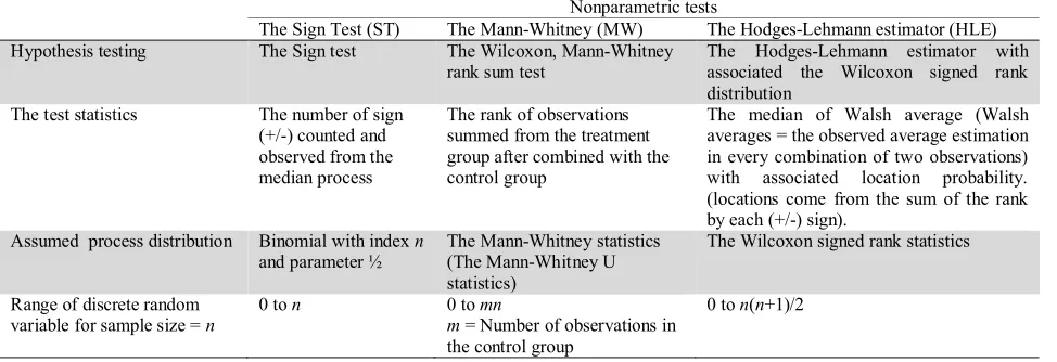
Table 1

The three nonparametric tests

Nonparametric tests

The Sign Test (ST) The Mann-Whitney (MW) The Hodges-Lehmann estimator (HLE) Hypothesis testing The Sign test The Wilcoxon, Mann-Whitney

rank sum test

The Hodges-Lehmann estimator with associated the Wilcoxon signed rank distribution

The test statistics The number of sign (+/-) counted and observed from the median process

The rank of observations summed from the treatment group after combined with the control group

The median of Walsh average (Walsh averages = the observed average estimation in every combination of two observations) with associated location probability. (locations come from the sum of the rank by each (+/-) sign).

Assumed process distribution Binomial with index n

and parameter ½

The Mann-Whitney statistics (The Mann-Whitney U statistics)

The Wilcoxon signed rank statistics

Range of discrete random variable for sample size = n

0 to n 0 to mn

m = Number of observations in the control group

0 to n(n+1)/2

3.2 Nonparametric control charts

The three nonparametric control chartings are compared in Table 2, the control limits of both ST and MW come from the Sign test and the Mann-Whitney statistics respectively, but only HL, for the control limits, uses the median of Walsh averages at the determined Wilcoxon signed rank locations. For the known process distribution, the probability distribution of the order statistics can be derived from the location of that order (Gibbons, 1971) (For example, the median is always at the middle of data), but not for the HLE because the median of Walsh average estimator is not always formed from the observations at the same ranks. Instead, the HLE depends on the magnitude of the two observations. Without the probability distribution function of HLE, the HL associates the HLE to the Wilcoxon signed rank distribution in constructing the control limits (Alloway et al., 1991).

Table 2

The three nonparametric control charts

Nonparametric control chart

The Sign Test (ST) The Mann-Whitney (MW) The Hodges-Lehmann estimator (HL)

Sample size N n (m for control group) n

Control limits Lower = -k

Upper = +k

aI+[0,n] +k = n-a

–k = a

aI+[0,mn] +k = mn-a

–k = a

aI+[0,n(n+1)/2]

+k = the median of Walsh average at

n(n+1)/2-a

–k = the median of Walsh average at a

Type I error () Binomial distribution  = Probability ( S+_<-_k_or

S+>+k )

Mann-Whitney U distribution

 = Probability (UT<-k or

UT>+k )

Wilcoxon signed rank distribution (WSR)  = Probability (WSR<a or

WSR>n(n+1)/2-a)

Test statistics, T S+ UT HE

Out of control condition S+<-k or S+>+k UT<-k or UT>+k HE <-k or HE>+k

The test statistics,T

The Sign test, S+

Suppose that x1, x2,…, xn is a random sample of size n from a continuous distribution with the median of the distribution, .

= ( − ) for i=1,2,…, n

(5)

where ( − ) = _0,1 , ₋− > 0



= 0

The random variable gives the number of positive signs in a sample and it has a Binomial distribution with parameters n and p=P(xi> ).

The Mann-Whitney, UT

Suppose that x1, x2,…, xn is a random sample of n elements from the treatment group, and y1, y2,…, ym

is a random sample of m elements from the control group,

x1,x2,…, xn,y1,y2,…, ym are random samples of size n+m.

Let MW ={x1,x2,…, xn, y1,y2,…, ym}, and

MW = sorted elements of MW in ascending order.

If Ri is the rank of the ith element of MW,

then Rt = ∑ is the sum of n treatment ranks.

UT = Rt - n(n+1)/2 . (2)

0 UTmn.

UT is called the Mann-Whitney statistics, and the statistics Rt is originated by Wilcoxon (Beaumont &

Knowles, 1996).

The Hodges-Lehmann estimator,HE

Suppose that x1, x2,…, xn is a random sample of size n from a continuous distribution.

Let Q = n(n+1)/2 The Walsh averages,

Wk=(xi+xj)/2 for k = 1,2, … ,Q

i < j

i = 1,2, … , n j = 1,2, … , n

HE =

if Q is odd ( + )/2 if Q is even

(3)

where,

d = (Q − 1)/2 if Q is odd

Q/2 if Q is even.

3.3 Control chart performance

(6)

The performance of the control charts are the in control average run length (ARL0) and the out of

control average run length (ARL1). When Type-I error = and Type-II error =, then

ARL0 =1/ (4)

ARL1=1/(1-). (5)

ARL0 represents the average number of samples that fall within the control limits before an out of

control condition occurs. ARL1 represents the average number of samples that is counteduntil the first

sample falls out of control limits when the process goes out of control (the mean shifts). Once the Type-I error () is known, ARL0 can be computed directly by equation (1) which is the performance by

usingformula. Therefore, by definition, ARL0 of the nonparametric control charts have the same result

for every underlying process distribution. ARL0 and ARL1 can also be computed by simulating the

samples from the given distribution for the in control (process mean = ) when the shifts occur (process mean = +).

The dual scheme for variable parameters control chart with variable sampling intervals (h), sample sizes (n), and control limits (action and warning limits (k and w)) are introduced. The continuous process starts from the Scheme 1 (n1,h1,k1,w1).The next sample will be drawn by the Scheme 1, if the previous sample is plotted in the central region [-w,+w]. The next sample will be drawn by the scheme 2 (n2,h2,k2,w2), if the previous sample is plotted in the warning regions [-k,-w) or (+w,+k]. The performances of the dual scheme for variable parameters control charts are as follows (Lin & Chou, 2007).

The average number of samples to signal (ANSS) is defined as the expected value of the number of samples taken from the start of the process to the time when the chart indicates out of control signal.

The average number of observation to signal (ANOS) is defined as the expected value of the number of observations taken from the start of the process to the time when the chart indicates out of control signal.

The average time to signal (ATS) is defined as the expected value of time from the start of the process to the time when the chart indicates out of control signal.

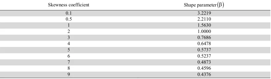
Table 3

Skewness coefficient and shape parameter of standard Weibull distribution (the scale parameter 1)

Skewness coefficient Shape parameter

0.1 3.2219

0.5 2.2110

1 1.5630

2 1.0000

3 0.7686

4 0.6478

5 0.5737

6 0.5237

7 0.4873

8 0.4596

9 0.4376

3.4 Process data

The process distributions in this study are the standard normal distribution (N(0,1)) and the standard Weibull distribution (the scale parameter  = 1).

(7)

A Weibull distribution has two parameters viz.,  and  where the value of skewness is inversely proportional to the shape parameter . Nelson (1979) as cited in Pongpullponsak et al. (2004) computed the parameter  for the skewness coefficient from 0.1, 0.5, 1, 2, …, 9 for =1 as shown in Table 3.

The performance in term of average run length (ARL) of the three control charts for the symmetry standard normal distribution, the 11 positive skewed (more data in the right elongated tail would be expected in the normal distribution) from symmetry to asymmetry shapes of standard Weibull distribution, and the process mean shifts in  times of standard deviation ( = 0, 0.25, 0.50, 0.75, 1, 1.5, 2, 2.5, and 3) will be compared to investigate; which chart is the most effective within the various experiment cases. The sample sizes are 10, 10,11,12,… , 20 for the Sign test control chart and the Hodges-Lehmann estimator control chart. For the Mann-Whitney control chart, the sample sizes are only in control group m = 10 and the treatment groups are n = 10, 11, 12, … ,15 due to the availability of statistical table (Beaumont & Knowles, 1996). The sample sizes n start from 10 because the statistics for control limits can be small enough and correspond to the Type-I error (), at least less than or equal to 0.0027 for 3 control limits of the normal data.

3.5 Simulation steps

The simulation methods for the average run length estimation are described as follows:

Step 1 Determine the control statistics for lower and upper action limits (-k, +k) and correspond to the

desired  probability.

Step 2 Compute the 10000 run lengths

Let RLi be the ith run length and given that RLi = 0 for i= 1 to 10000

[a] For each RLi

[b] – Generate the random number xi for i=1,2, …,n (the sample size =n) from the given

distribution with the process parameter +

- Compute the statistic



- Compare the statistic T with control limits

If -k T +k then RL = RL + 1 and go to [b]

If T< -k or T> +k, then if  = 0, RLi= RL

else if  > 0, RLi = RL+1.

set RL = 0 and go to [a]

Step 3 Compute the average run length

= ∑ ₁₀₀₀₀ (6)

For the Mann-Whitney statistics, the control group of sample size m also generates randomly from the in control process with mean = +0.

The Hodges-Lehmann estimator control limits come from Walsh averages at the determined Wilcoxon signed rank locations (Das, 2009). The simulation method for HL control limits is described as follows:

Step 1 Determine the Wilcoxon signed rank statistics for lower and upper control limits

Step 2 Compute 100000 sets of Walsh averages of the sample size n from the given distribution with

(8)

Step 3 Compute the median of Walsh averages at the determined Wilcoxon signed rank locations for

lower and upper control limits

All models in this study are designed in MATLAB using custom scripts.

4. Results and discussion

The results of the Sign test (ST), the Mann-Whitney (MW), and the Hodges-Lehamann estimator (HL) control charts for the normal dataand Weibull data are presented as follows.

4.1 The Sign test control charts

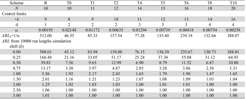
Twelve fixed parameter Sign test control charts with sample sizes from 10,10,11, …, 20, determined control limits with  closed to 0.0027 (closed to 3 control limits in Shewhart chart) denoted by–k and +k for action limits, and ARL0 and ARL1 of selected schemes for standard normal data are shown in Table 4. The ARL0 from both  and the simulation are in the same magnitude i.e., for n=10 in the

scheme R,  = 0.00195, ARL0 from  =512, and ARL0 from simulation = 508.01.

The dual scheme for variable parameters control charts is set from the schemes in Table 4.

Table 4

Average run length of the Sign test control chart for standard normal data

Scheme R T0 T1 T2 T4 T5 T6 T8 T10

N 10 10 11 12 14 15 16 18 20

Control limits

+k 9 8 9 10 11 12 13 14 16

-k 1 2 2 2 3 3 3 4 4

 0.00195 0.02148 0.01172 0.00635 0.01294 0.00739 0.00418 0.00754 0.00258

ARL0=1/ 512.00 46.55 85.33 157.54 77.28 135.40 239.18 132.66 388.07

ARL from 10000 run lengths simulation shift ()

0.00 508.01 45.12 83.94 158.80 76.15 136.39 235.67 130.73 388.01

0.25 166.48 21.16 33.05 51.17 25.24 37.34 55.04 31.12 64.93

0.50 39.83 7.36 9.63 12.99 6.90 8.79 11.52 6.87 10.80

0.75 13.17 3.30 3.97 4.87 2.85 3.28 3.86 2.56 3.31

1.00 5.56 1.92 2.17 2.43 1.63 1.79 1.90 1.47 1.65

1.50 2.01 1.16 1.21 1.23 1.07 1.08 1.09 1.03 1.04

2.00 1.25 1.02 1.03 1.03 1.00 1.01 1.01 1.00 1.00

2.50 1.06 1.00 1.00 1.00 1.00 1.00 1.00 1.00 1.00

3.00 1.01 1.00 1.00 1.00 1.00 1.00 1.00 1.00 1.00

The result shows that the regular scheme is equal to the scheme R and the tight scheme, which is smaller in central region and larger in both warning and out of control regions, when comparing to the scheme R, from T0 (tighter than R), T1, T2, T4, T5, T6, T8, and T10 as shown in Table 5. The performance of ANSS, ANOS, and ATS of the dual scheme for variable parameters Sign test control chart for the normal data are computed by 10000 runs simulation, as shown in Table 5. The ANSS of each VP scheme shows the weighted average from ARLs of the combined schemes that are reduced from the ARL of the regular principal scheme R in every combination.

(9)

Table 5

ANSS, ANOS, and ATS from 10000 runs simulation of Variable parameters Sign test control chart for standard normal data (n1=10, h1=1)

VP Scheme R&R R&T0 R&T1 R&T2 R&T4 R&T5 R&T6 R&T8 R&T10

n2 10 10 11 12 14 15 16 18 20

h2 0.5 0.5 0.5 0.5 0.5 0.5 0.5 0.5 0.5

+k 9 8 9 10 11 12 13 14 16

+w 7 6 7 8 9 10 10 11 13

-w 3 4 4 4 5 5 6 7 7

-k 1 2 2 2 3 3 3 4 4

central 0.89063 0.65625 0.77344 0.85400 0.82043 0.88153 0.69824 0.76212 0.88468 warning 0.10742 0.32227 0.21484 0.13965 0.16663 0.11108 0.29758 0.23035 0.11274 shift () ANSS

0.00 505.02 211.14 313.88 405.26 308.58 392.23 452.92 378.16 494.88 0.25 167.21 63.16 90.72 117.29 77.28 101.72 118.05 83.73 125.94 0.50 39.40 11.72 16.29 21.43 12.18 15.46 17.09 10.21 17.08 0.75 12.22 3.39 4.19 5.39 2.91 3.55 3.72 2.33 3.24 1.00 4.75 1.56 1.75 2.06 1.34 1.46 1.52 1.17 1.32 1.50 1.50 1.02 1.04 1.05 1.01 1.01 1.01 1.00 1.00 2.00 1.05 1.00 1.00 1.00 1.00 1.00 1.00 1.00 1.00 2.50 1.00 1.00 1.00 1.00 1.00 1.00 1.00 1.00 1.00 3.00 1.00 1.00 1.00 1.00 1.00 1.00 1.00 1.00 1.00 shift () ANOS

0.00 5050.16 2111.43 3176.79 4142.84 3227.40 4134.38 4853.18 4152.83 5484.97 0.25 1672.06 631.56 925.32 1215.50 831.55 1107.99 1326.15 981.68 1492.66 0.50 394.03 117.24 169.58 230.41 141.65 183.85 218.63 143.03 243.61 0.75 122.20 33.94 44.71 60.61 37.14 47.01 54.42 38.54 56.60 1.00 47.53 15.62 19.03 24.08 18.22 20.97 23.78 20.87 25.61 1.50 14.97 10.22 11.40 12.57 14.06 15.10 16.14 18.01 20.03 2.00 10.53 10.00 11.01 12.00 13.99 15.00 16.00 18.00 20.00 2.50 10.04 10.00 11.00 12.00 13.97 15.00 16.00 17.97 19.99 3.00 10.00 10.00 10.98 11.99 13.95 15.00 15.99 17.98 19.95 shift () ATS

0.00 505.02 196.58 294.87 382.69 290.87 371.02 425.92 354.96 468.06 0.25 167.21 56.00 81.69 106.64 69.94 92.64 105.91 74.71 114.28 0.50 39.40 9.04 12.93 17.40 9.70 12.54 13.12 7.65 13.45 0.75 12.22 2.17 2.77 3.71 1.91 2.39 2.29 1.37 2.03 1.00 4.75 0.86 0.99 1.20 0.73 0.82 0.80 0.60 0.69 1.50 1.50 0.51 0.52 0.53 0.50 0.51 0.50 0.50 0.50 2.00 1.05 0.50 0.50 0.50 0.50 0.50 0.50 0.50 0.50 2.50 1.00 0.50 0.50 0.50 0.50 0.50 0.50 0.50 0.50 3.00 1.00 0.50 0.51 0.50 0.51 0.50 0.50 0.50 0.50

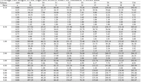
Table 6

Average run length of the Sign test control chart for standard Weibull data

Scheme shift R T0 T1 T2 T4 T5 T6 T8 T10

Skew n 10 10 11 12 14 15 16 18 20

0.10 0.00 510.51 45.38 84.44 155.15 75.56 134.89 234.64 134.05 393.93 0.25 176.69 22.17 34.35 53.94 26.78 39.96 59.66 33.39 70.69 0.50 44.14 7.96 10.66 14.25 7.41 9.80 12.55 7.39 11.97 0.75 14.33 3.51 4.33 5.25 3.07 3.54 4.16 2.73 3.62 1.00 6.11 2.04 2.26 2.57 1.69 1.86 2.03 1.52 1.72 1.50 1.98 1.15 1.20 1.23 1.07 1.08 1.10 1.03 1.04 2.00 1.18 1.01 1.01 1.01 1.00 1.00 1.00 1.00 1.00 2.50 1.02 1.00 1.00 1.00 1.00 1.00 1.00 1.00 1.00 0.50 0.00 517.92 45.21 82.18 155.90 76.08 133.22 238.37 133.18 385.63

0.25 172.71 21.87 34.01 53.08 25.79 38.74 56.94 32.48 67.29 0.50 38.95 7.23 9.66 12.83 6.74 8.86 11.02 6.63 10.40 0.75 11.85 3.08 3.64 4.39 2.63 2.97 3.43 2.35 2.95 1.00 4.46 1.72 1.85 2.07 1.44 1.54 1.65 1.31 1.43 1.50 1.39 1.04 1.05 1.06 1.01 1.01 1.01 1.00 1.00 1.00 0.00 509.00 46.21 84.20 151.12 75.40 136.75 235.14 132.82 390.25

0.25 151.69 19.50 30.32 46.60 23.05 33.75 49.28 28.20 56.30 0.50 28.18 5.76 7.38 9.62 5.11 6.41 8.04 4.98 7.32 0.75 6.96 2.21 2.51 2.90 1.85 2.05 2.24 1.66 1.92 1.00 2.31 1.23 1.28 1.33 1.10 1.13 1.15 1.05 1.07 2.00 0.00 496.90 45.57 84.07 159.38 76.88 135.62 240.55 131.35 384.33

0.25 85.51 12.62 17.99 26.56 13.31 18.39 25.61 14.64 26.35 0.50 7.00 2.21 2.49 2.86 1.84 2.03 2.24 1.63 1.91 3.00 0.00 507.93 45.18 83.94 155.08 76.06 133.76 238.93 131.65 393.91

0.25 27.16 5.46 7.06 9.13 4.99 6.17 7.72 4.77 6.92 4.00 0.00 505.26 45.75 83.75 155.34 75.40 133.33 241.60 131.81 385.94

0.25 2.14 1.20 1.23 1.28 1.08 1.10 1.13 1.04 1.06 5.00 0.00 509.76 45.59 84.88 155.73 75.87 134.05 231.84 134.90 383.33 6.00 0.00 512.89 45.44 83.64 157.81 77.05 133.40 238.77 130.34 391.06 7.00 0.00 506.99 46.41 86.26 156.83 76.67 133.09 239.92 132.05 384.07 8.00 0.00 509.86 46.28 85.90 157.18 75.37 135.36 240.41 132.61 387.28 9.00 0.00 497.29 45.48 84.42 154.67 76.28 135.60 237.70 132.30 383.87

(10)

4.2 The Mann-Whitney control charts

From the available Mann-Whitney distribution table (Beaumont & Knowles, 1996), seven fixed parameter Mann-Whitney control charts with sample sizes from control group m = 10 and the treatment group n = 10,10,11, …, 15, determined control limits with  closed to 0.0027 (closed to 3 control limits in Shewhart chart) denoted by –k and +k for action limits, and ARL0 and ARL1 of selected

schemes for standard normal data are shown in Table 7.

Table 7

Average run length of the Mann-Whitney control chart for standard normal data

Scheme R T0 T1 T2 T3 T4 T5

Control, m 10 10 10 10 10 10 10

Treament, n 10 10 11 12 13 14 15

Control limits

+k 88 87 95 102 110 118 126

-k 12 13 15 18 20 22 24

Mann-Whitney U statistics probability

89-100 0.00104 0.00144 0.00138 0.00172 0.00162 0.00153 0.00145 0-11 0.00104 0.00144 0.00138 0.00172 0.00162 0.00153 0.00145

 0.00208 0.00288 0.00276 0.00344 0.00324 0.00306 0.00290

ARL0=1/ 480.77 347.22 362.32 290.70 308.64 326.80 344.83

Shift() Within action limits = control group data come from within action limits only

0.00 476.39 347.39 367.99 295.24 306.85 328.65 346.61 0.25 203.10 152.32 152.46 120.92 122.10 123.56 130.21

0.50 56.04 45.86 42.86 34.50 34.33 33.80 33.73

0.75 19.44 15.94 14.69 12.08 11.59 11.40 11.06

1.00 8.10 6.77 6.25 5.16 4.99 4.94 4.77

1.50 2.44 2.19 2.03 1.79 1.74 1.69 1.66

2.00 1.31 1.25 1.20 1.15 1.12 1.11 1.09

2.50 1.05 1.04 1.03 1.02 1.01 1.01 1.01

3.00 1.00 1.00 1.00 1.00 1.00 1.00 1.00

Shift() Without action limits restriction for control group data

0.00 472.93 352.06 363.07 291.95 306.23 325.90 340.10 0.25 205.13 153.10 151.64 122.20 126.56 128.07 129.00

0.50 58.03 45.02 43.35 34.50 33.71 33.18 34.15

0.75 19.44 15.81 15.02 11.98 11.67 11.45 11.26

1.00 8.19 6.89 6.43 5.28 5.11 4.87 4.77

1.50 2.46 2.22 2.05 1.82 1.76 1.70 1.66

2.00 1.32 1.25 1.22 1.15 1.14 1.12 1.11

2.50 1.06 1.04 1.03 1.02 1.01 1.01 1.01

3.00 1.01 1.00 1.00 1.00 1.00 1.00 1.00

Table 7 shows that there were nearly the same between ARL from Type-I error () and the ARL from 10000 runs simulation for the normal data when control group sample data come from +0 process parameter within only control limits and there was no restriction about the other methods.

Table 8

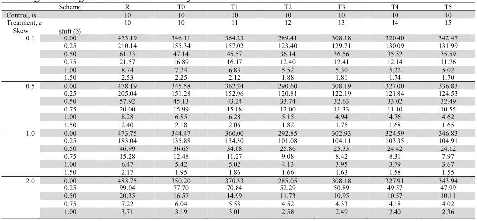
Average run length of the Mann-Whitney control chat for standard Weibull data

Control, m 10 10 10 10 10 10 10

Treatment, n 10 10 11 12 13 14 15

Skew shift ()

0.1 0.00 473.19 346.11 364.23 289.41 308.18 320.40 342.47 0.25 210.14 155.34 157.02 123.40 129.71 130.09 131.99 0.50 61.33 47.14 45.57 36.14 36.56 35.52 35.59 0.75 21.57 16.89 16.17 12.40 12.41 12.14 11.76

1.00 8.74 7.24 6.83 5.52 5.30 5.22 5.02

1.50 2.53 2.25 2.12 1.88 1.81 1.74 1.70

0.5 0.00 478.19 345.58 362.24 290.60 308.19 327.00 336.83 0.25 205.04 151.28 152.96 120.81 122.19 121.84 124.53 0.50 57.92 45.13 43.24 33.74 32.63 33.02 32.49 0.75 20.00 15.99 15.08 12.00 11.33 11.10 10.55

1.00 8.28 6.85 6.28 5.15 4.94 4.76 4.62

1.50 2.40 2.18 2.06 1.82 1.75 1.68 1.65

1.0 0.00 473.75 344.47 360.00 292.85 302.93 324.59 346.83 0.25 183.04 135.88 134.30 101.08 104.11 103.35 104.91 0.50 46.99 36.65 34.08 25.86 25.33 24.42 24.12

0.75 15.28 12.48 11.27 9.08 8.42 8.31 7.97

1.00 6.47 5.42 5.02 4.13 3.95 3.79 3.67

1.50 2.17 1.95 1.86 1.66 1.63 1.58 1.55

2.0 0.00 483.75 350.20 370.33 285.05 308.18 327.91 343.94 0.25 99.04 77.70 70.84 52.29 50.89 49.57 47.99 0.50 20.35 16.57 14.99 11.73 10.95 10.57 10.11

0.75 7.22 6.04 5.53 4.52 4.33 4.18 4.02

(11)

The ARLs result from 10000 runs simulation for standard Weibull data is shown in Table 8. The dual scheme for variable parameters Mann-Whitney control charts for both normal and Weibull data also show the combination results, as the same result having ever happened in the normal data. However, the shift rows that all ARL≤2 are not shown in the table.

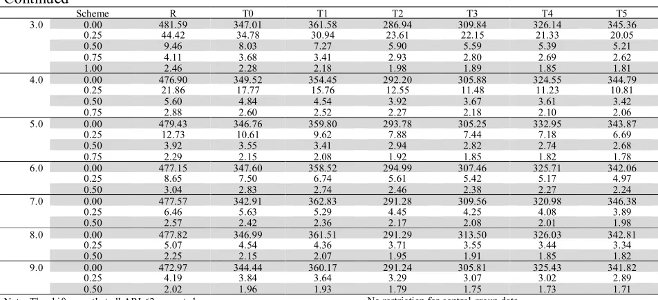
Table 8 Continued

3.0 0.00 481.59 347.01 361.58 286.94 309.84 326.14 345.36

0.25 44.42 34.78 30.94 23.61 22.15 21.33 20.05

0.50 9.46 8.03 7.27 5.90 5.59 5.39 5.21

0.75 4.11 3.68 3.41 2.93 2.80 2.69 2.62

1.00 2.46 2.28 2.18 1.98 1.89 1.85 1.81

4.0 0.00 476.90 349.52 354.45 292.20 305.88 324.55 344.79

0.25 21.86 17.77 15.76 12.55 11.48 11.23 10.81

0.50 5.60 4.84 4.54 3.92 3.67 3.61 3.42

0.75 2.88 2.60 2.52 2.27 2.18 2.10 2.06

5.0 0.00 479.43 346.76 359.80 293.78 305.25 332.95 343.87

0.25 12.73 10.61 9.62 7.88 7.44 7.18 6.69

0.50 3.92 3.55 3.41 2.94 2.82 2.74 2.68

0.75 2.29 2.15 2.08 1.92 1.85 1.82 1.78

6.0 0.00 477.15 347.60 358.52 294.99 307.46 325.71 342.06

0.25 8.65 7.50 6.74 5.61 5.42 5.17 4.97

0.50 3.04 2.83 2.74 2.46 2.38 2.27 2.24

7.0 0.00 477.57 342.91 362.83 291.28 309.56 320.98 346.38

0.25 6.46 5.63 5.29 4.45 4.25 4.08 3.89

0.50 2.57 2.42 2.36 2.17 2.08 2.01 1.98

8.0 0.00 477.82 346.99 361.51 291.29 313.50 326.03 342.81

0.25 5.07 4.54 4.36 3.71 3.55 3.44 3.34

0.50 2.25 2.15 2.07 1.95 1.91 1.85 1.82

9.0 0.00 472.97 344.44 360.17 291.24 305.81 325.43 341.82

0.25 4.19 3.84 3.64 3.29 3.07 3.02 2.89

0.50 2.02 1.96 1.93 1.79 1.75 1.73 1.71

Note: The shift rows thatall ARL2 are not shown. No restriction for control group data.

4.3 The Hodges-Lehmann estimator control charts

The ARL performed by 10000 run lengths simulation of the Hodges-Lehmann estimator control chart for the normal data shows very high ARL when comparing to the ARL0 from the Wilcoxon signed rank

statistics. The control limits, proposed byAlloway et al. (1991), are computed by the original method as shown in Table 9. For the sample size n =10, (-k,+k) = (2,53),  = 0.00390, ARL0 = 256.41, the

median of Walsh averagesfor 100000 samples simulation at (2,53) are (-1.50027, 1.15015), by using this Hodges-Lehmann control limit the ARL0 from 10000 run lengths simulation = 4241.49. The control

limits (-1.50027, 1.15015) has the probability= 0.7703 in N(0,1),  = 0.2297, ARL0 =4.35. For the

sample size n = 10, using the Wilcoxon signed rank wider control limits at (1, 54) with the probability

 = 0.00196, ARL0 = 510.20, it shows that the ARL0 performance is better than 3 control limit,

=0.0027, ARL0 = 370 in Shewhart chart, and HL control limits from 100000 sets of Walsh

averages= (-1.4993, 1.2544) with the probability = 0.8283 in N(0,1),  = 0.1717, ARL0 from process

distribution =5.82, but the ARL0 from 10000 run lengths simulation = 13281.35 (this case is not shown

in Table 9). For the known process distribution, the robust to outliers of the Hodges-Lehmann estimator give this very high ARL performance. The Hodges-Lehmann estimator is the nonparametric statistics that is very robust to the presence of outliers (Duchnowski, 2013).

For the original HL method, the sample size in HL must be started from 10 in order that the Type-I error probability is low enough (ARL0 is high enough) from Wilcoxon signed rank statistics. But for the

normal data, ARL0 in the simulation is about 3 to 16 times of ARL0 from Wilcoxon signed rank

probability. The very high ARL0 in the simulation leads to a chance in using the smaller sample size n

(12)

Table 9

Average run length of the Hodges-Lehmann estimator control chart for standard normal data using the original charting technique

n 10 10 11 12 14 15 16 18 20

n(n+1)/2 55 55 66 78 105 120 136 171 210

Wilcoxon Signed Rank Statistic action limits

+k 53 51 63 73 96 108 121 150 181

-k 2 4 3 5 9 12 15 21 29

 0.00390 0.00896 0.00292 0.00342 0.00306 0.00336 0.00336 0.00280 0.00272

ARL0 =1/ 256.41 111.61 342.47 292.40 326.80 297.62 297.62 357.14 367.65

Hodges-Lehmann Estimator Control Limits from 100000 runs simulation

+k 1.15015 1.14950 1.09318 1.01846 0.93124 0.87789 0.84133 0.80215 0.76000 -k -1.50027 -1.25569 -1.20516 -1.08337 -0.97378 -0.91128 -0.87195 -0.82538 -0.77042 ARL from 10000 run lengths simulation

Shift ()

0.00 4241.49 3260.34 3401.88 2102.92 1642.85 1227.30 1079.72 1224.29 1132.42 0.25 328.55 322.06 288.14 197.77 145.20 108.76 91.24 86.50 74.70

0.50 42.46 41.96 35.19 24.28 16.96 12.71 10.68 9.33 7.76

0.75 8.90 9.05 7.45 5.43 3.88 3.15 2.76 2.39 2.06

1.00 3.13 3.06 2.61 2.09 1.69 1.47 1.37 1.26 1.17

1.50 1.16 1.17 1.11 1.06 1.02 1.01 1.00 1.00 1.00

Note: The shift rows thatARL 1 are not showed.

The new approach to find the right performance for the known process distribution is using the Hodges-Lehmann estimator at the locations corresponding to the desired Type-I error probability as the control limits. To verify with 3 control limits of Shewhart chart,  = 0.00270, ARL0 = 370.37), in

the new approach to HL, for n = 10, Type I error () = 0.00270, –k = 135 and +k = 99865 are the locations of control limits from the 100000 ascending order simulated Hodges-Lehmann estimator and they are the new Hodges-Lehmann control limits (-0.99573, 0.99179) with ARL0 from 10000 run

lengths simulation = 401.03. The 401.03 is also closed to 370.

The Hodges-Lehmann estimator control chart for the normaldata by using the new control limits for Type-I error probability =0.0027 (ARL0 =370.37) with selected sample sizes from 10 to 20 present in

Table 10.

Table 10

Average run length of the new Hodges-Lehmann estimator control chart for standard normal data

Scheme Rs Ts Rs1 Rs2 Rs3 Rs4 Rs5

n 10 10 11 12 13 14 15

Type I error () 0.00270 0.00308 0.00270 0.00270 0.00270 0.00270 0.00270 Location at

+k 99865 99845 99865 99865 99865 99865 99865

-k 135 155 135 135 135 135 135

Hodges-Lehmann estimator control limits from 100000 runs simulation

+k 0.99179 0.97489 0.92749 0.89708 0.86389 0.82901 0.78779

-k -0.99573 -0.97909 -0.93255 -0.90214 -0.87512 -0.82383 -0.79610

ARL from 10000 run lengths simulation shift ()

0.00 401.03 342.40 345.64 376.66 402.13 362.69 336.38

0.25 84.20 74.51 66.80 67.60 61.94 55.49 46.29

0.50 15.03 13.53 11.72 10.93 9.65 8.49 7.08

0.75 4.42 3.99 3.55 3.21 2.93 2.63 2.22

1.00 1.96 1.88 1.70 1.57 1.48 1.36 1.26

1.50 1.06 1.05 1.03 1.02 1.01 1.01 1.00

2.00 1.00 1.00 1.00 1.00 1.00 1.00 1.00

2.50 1.00 1.00 1.00 1.00 1.00 1.00 1.00

3.00 1.00 1.00 1.00 1.00 1.00 1.00 1.00

When the sample size is increasing the control limits is also narrower, the sample size affects the control limits vis-à-vis 1/√n in the Shewhart chart, and the ARL0 of each scheme from simulation

are 370 (in the range of401 to 336). The tight control by using = 0.00308 (ARL0 = 324.37) for the

Scheme Ts isin Table 10, and ARL0 from the simulation= 342.40. The ARL0 from the simulation in this

new control limits does not show the very high value as the original practice presented in Table 9.

(13)

presented. The dual scheme for variable parameters control charts of the Hodges-Lehmann estimator control charts for both the normal and Weibull data also show the combination results for performances of ANSS, ANOS, and ATS, the same results as having ever happened in the Sign test control charts. However, the table is not presented.

5. Conclusion

The performances of the three nonparametric control charts (ST, MW, and HL) for the known process distribution (normal and Weibull data) shown inthis simulation study are as follows.

The control limits of the three nonparametric control charts are not effected from the sample sizes (1/√n in chart), but the Type-I error () probability is associated with the selected non-parametric statistics for only control limits. In the Sign test and the Mann-Whitney control charts, the ARL0

performance follows the Type-I error probability () from the control statistics. For only the original Hodges-Lehmann estimator control chart, the robust to outliers of the median of Walsh averages also gives narrower control limits and the simulation also shows very large ARL performance when compared to the ARL performance from the Type-I error probability () which is derived from the assumed Wilcoxon signed rank statistics.

The new HL approach by using the control limits derives from the Hodges-Lehmann estimator distribution, and the ARL performance shows the effect of increasing sample size as the effect of 1/√n

in the Shewhart chart. At the 3 control limits in the normal data, the ARL0 of this new control

limits also closesto 370 as that inthe Shewhart chart.

For the variable parameters, the performance of the combined dual schemes is the weighted averages between the regular scheme and the tight scheme in every non-parametric control chart.

In term of the Hodges-Lehmann estimator control chart for the known process distribution, the control limits at the given probability can be derived by the simulation, then the HL will be the alternative method for the process that needs the robust to outlier property from this statistics, and it is possible that the economic design (expected costs per unit time) will be solved.

References

Alloway, J.A. & Raghavachari, M. (1991). Control chart based on Hodges–Lehmann estimator.

Journal of Quality Technology, 23, 336–347.

Amin, R.W., &Widmaier, O. (1999). Sign control charts with variable sampling intervals.

Communication in Statistics - Theory and Methods, 28(8), 1961–1985.

Amin, R., Reynolds Jr, M.R., & Bakir, S.T. (1995).Nonparametric quality control charts based on the sign statistic.Communication in Statistics - Theory and Methods, 24, 1579–1623.

Bakir, S.T. (2001). Classification of distribution-free quality control charts, Proceedings of the Annual Meeting of the American Statistical Association, August 5-9, 2001.

Bakir, S.T. (2004). A distribution-free Shewhart quality control chart based on Signed-rank. Quality

Engineering, 16(4),613-623.

Bakir, S.T. & Reynolds, M.R. (1979).A nonparametric for process control based on within-groups ranking. Technometrics, 21(2), 175-183.

Balakrishnan, N., Triantafyllou, I.S. & Koutras, M.V. (2009). Nonparametric control charts based on runs and Wilcoxon-type rank-sum statistics. Journal of Statistical Planning and Interface, 139, 3177-3192.

Beaumont, G.P., & Knowles, J.D. (1996). Statistical tests An introduction with MINITAB commentary. Hertfordshire: Prentice Hall international (UK) Limited.

(14)

Black, G., Smith, J. & Wells, S. (2011). The impact of Weibull data and autocorrelation on the performance of the Shewhart and exponentially weighted moving average control charts.

International Journal of Industrial Engineering Computations, 2, 575-582.

Bluman, A.G. (1998). Elementary Statistics : a step by step approach. Boston: WCB McGraw-Hill. Chakraborti, S.&Eryilmaz, S. (2007). A nonparametric Shewhart-type signed-rank control chart based

on runs.Communications in Statistics – Simulation and Computation, 36(2), 335-356.

Chakraborti, S., van der Lann, P., & Bakir, S.T. (2001). Nonparametric control charts: an overview and some results. Journal of Quality Technology, 33(3), 304-315.

Chakraborti, S. & van de Wiel, M.A. (2008).A nonparametric control chart based on the Mann-Whitney statistic.IMS Collections. Institute of Mathematical Statistics, 1, 156–172.

Cheng, A.Y., Liu, R.Y. & Luxhoj, J.T. (2000).Monitoring Multivariate Aviation Safety Data by Data Depth: Control Charts and Threshold Systems. IIE Transactions, 32, 861-872.

Das, N. (2009). A comparison study of three non-parametric control charts to detect shift in location parameters. The International Journal of Advanced Manufacturing Technology, 41, 799-807.

Duchnowski R. (2013). Hodges–Lehmann estimates in deformation analyses. Journal of

Geodynamics, 87, 873–884.

Ghute, V.B. & Shirke, D.T.(2012). A nonparametric Signed-rank control chart for bivariate process location. Quality Technology & Quantitative Management, 9(4), 317-328.

Gibbons, J.D. (1971). Nonparametric Statistical Inference. Tokyo: McGraw-Hill Kogakusha.

Graham, M.A., Human, S.W. & Chakraborti, S. (2010). A phase I nonparametric Shewhart-type control chart based on the median. Journal of Applied Statistics, 37(11), 1795-1813.

Graham, M.A., Chakraborti, S., & Human, S.W. (2011).A nonparametric exponentially weighted moving average signed-rank chart for monitoring location. Computational Statistics and Data

Analysis, 55, 2490-2503.

Graham, M.A., Mukherjee, A. & Chakraborti, S. (2012). Distribution-free exponentially weighted moving average control charts for monitoring unknown location. Computational Statistics and Data

Analysis, 56, 2539-2561.

Human, S.W., Chakraborti, S. & Smit, C.F. (2010).Nonparametric Shewhart-type Sign control charts based on runs. Communication in Statistics - Theory and Methods, 39(11), 2046–2062.

Jones-Farmer, L.A., Jordan, V. & Champ, C.W. (2009). Distribution-free phase I control charts for subgroup location. Journal of Quality Technology, 41(3), 304-316.

Khilare, S.K., & Shirke, D.T. (2010). A nonparametric synthetic control chart using Sign statistic.

Communicatins in statistics – Theory and Methods, 39(18), 3282-3293.

Lehmann, E.L. (1963). Non-parametric confidence intervals for a shift parameter. The Annals of

Mathematical Statistics, 34, 1507–1512.

Li, J., Zhang, X. & Jeske, D.R. (2013).Nonparametric multivariate CUSUM control charts for location and scale changes. Journal of Nonparametric Statistics, 25(1), 1-20.

Lin, Y.C. & Chou, C.Y. (2007). Non-normality and the variable parameters control charts. European

Journal of Operations Research, 176, 361-373.

Montgomery, D.C. (2013). Statistical quality control (7th edition). Asia: John Wiley & Sons Singapore.

Nelson, P.R. (1979). Control Charts for Weibull Processes with Standards Given. IEEE Transactions

on Reliability, 28, 283-288.

Neuhäuser, M. (2012). Nonparametric Statistical tests: A computational Approach. Florida : CRC Press.

Pongpullponsak, A., Suracherdkiati, W., & Kriweradechachai, P. (2004). The comparison of efficiency of control chart by weighted variance method, Nelson Method, Shewhart method for skewed population, Proceeding of the 5th Applied Statistics Conference of Northern Thailand; 2004 May 27-29; Chiang Mai, Thailand.

The Math WorksTM. (2009). MATLAB 7.6.0(R2009a). License Number 350306, February 12, 2009. Yang, S., Lin, J., & Cheng, S.W. (2011). A new nonparametric EWMA Sign Control Chart. Expert