Abduction as Incomplete Parameter Estimation

Abduction as Incomplete Parameter Estimation

Moto Kamiura

[email protected], [email protected], Faculty of Science and Technology, Tokyo University of Science, Japan

Abstract: Abduction is a kind of logical inference, and has been studied in computer science and artificial intelligence (Fin-lay and Dix 1996). Recently, Sawa and Gunji (2010) introduced a diagram to represent three types of inference: i.e. deduc-tion, inducdeduc-tion, and abducdeduc-tion, which are articulated by C.S.Peirce. Sawa-Gunji’s representation provides a new approach to a numerical aspect of abduction. In the present paper, we show that Sawa-Gunji's representation of abduction is consistent with Finlay-Dix's one, and integrate the two representations. Both parameter estimation and abduction occupy a similar position on the integrated representation, although they are not completely corresponding. We present "incomplete" pa-rameter estimation as a sort of "simulated abduction", which is a numerical aspect of abduction. It is applied to a first-order autoregressive (AR(1)) model. As a result of numerical analyses on AR(1), the incompletely estimated parameter (IEP) follows a Cauchy distribution, which has a power law of the slope -2 in the tail, although conventionally estimated parameter is normally distributed. It is shown that the Cauchy distribution of the IEP is based on structure of ratio distribution of normal random variables generated from the AR(1). This research suggests that the distribution of the IEP is not based on a mech-anism of system itself, but on relationship between data structure on the given system (i.e. the given AR(1) process) and one on the system observer (i.e. the estimator of the AR(1) parameter).

Keywords: Autoregressive model, Parameter Estimation, Observation, Cauchy distribution, Power law

Acknowledgement: Part of this work was carried out under the Cooperative Research Project Program of the Research Institute of Electrical Communication, Tohoku University.

1.

Introduction

C.S. Peirce who is a philosopher/logician classifies reasoning/inference into three types: i.e. deduc-tion, induction and abduction (Peirce 1868; 1955). Abduction has been studied not only in philoso-phy but also in artificial intelligence and computer science (Bylander et al 1991; Tanner and Jo-sephson 1996; Finlay and Dix, 1996; Abe 2003). Recently, Sawa and Gunji presented a model representing dynamic change in logical inference (Sawa and Gunji 2010). To define the model dynamics, they propose an arrow diagram which is a tool to illustrate each of the three types of inference. Sawa-Gunji’s representation of abduction is an operation in which an arrow in the dia-gram is derived from the other arrows. This formalization for abduction is not only consistent with the preceding studies (Peirce 1868; Finlay and Dix 1996), but also provides a new approach to a numerical aspect of abduction (Kamiura 2010).

In the present paper, inheriting the Sawa-Gunji’s representation, we formalize a numerical as-pect of abduction and find “incomplete” parameter estimation as a sort of “simulated abduction”. Auto-regressive (AR(1)) model is used for numerical experiments and the results are shown. In the conclusion, we discuss abduction mediating a relationship between system observer and power law distributions.

2.

Diagrams of Inference and Positioning of Abduction

Abduction includes an intrinsic incompleteness, which means that abduction is formally equiva-lent to “the logical fallacy affirming the consequent”. Therefore, the context needs to be clearly de-scribed to avoid unnecessarily confusing.

Let us recall a representation of abduction by Finlay and Dix (1996). It has almost the same meaning which is given by Peirce (1955). Finlay and Dix use the representation of the first-order predicate logic,

, (1)

where a and b are predicates and x is a variable. In standard logic, given a proposition a(x0) with a

value x0, one can deduce b(x0) (i.e. deduction). In abduction, one deduces the inverse: i.e. if one

knows b(x0), then one deduces a(x0). This is not permitted in standard logic, but is a formalization of

abduction.

Recently, Sawa and Gunji (2010) introduced the following arrow diagram, Figure 1, to represent the three types of inference. Each inference is expressed as an operation in which one arrow is derived from the other two arrows on this diagram.

Figure 1: Sawa-Gunji’s representation for

inference.

Finlay-Dix’s representation and Sawa-Gunji’s one are consistent with each other. Let us express arrows of the Sawa-Gunji’s diagram by

a

:= Minor premise, f := Major premise and b: = Conclusion. When the arrow diagram is a commutative one and the dot on the lower left corner of the diagram is considered as a set of the variable x, we can obtain , which is equal to (1). The integration of Finlay-Dix’s representation and Sawa-Gunji’s one is expressed in Figure 2.

We can also confirm an example of conventional syllogism by the following substitution:

a

(

x

) = “

x

is a human”, f = “If

x

is a human, then

x

is mortal” (i.e. “humans are mortal”) and b

(

x

) = “

x

is mortal”.

Figure 2: Integration of the Finlay-Dix’s

representation and the Sawa-Gunji’s one.

In addition, we can see that abduction is accounted for by deriving the upper left arrow (i.e. “the minor premise” or the map

a

) on Figure 1 or 2.

3.

Transplanting Inference Structure to Numerical Function System

3.1.Modifying the Sawa-Gunji’s Representation

In this section, the diagram for logical inference in Figure 2 is converted into a diagram for numeri-cal numeri-calculations. The following restriction is proposed: i.e. restrict the map

a

in Figure 2 to a map (

α

,

Minor premise

Major premise

Conclusion

a

a

(

x

)

f

b

-

)

,

where

_α

is a parameter and the hyphen – is a blank space for which a value

x

is substituted

.

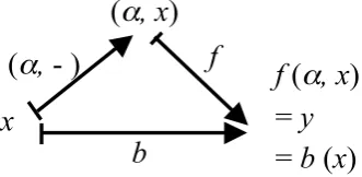
This procedure generates a diagram in Figure 3.

Figure 3: The diagram to transplant the structure of inference to numerical function system.

Each map in Figure 3 is interpreted as the following: (A1) the map adds

infor-mation of the premise (i.e. the parameter value

_α

) of system structure f to the input data x. (A2) the system transforms the input data x into the output data y, under the parameter

_α

. (A3) Composition of the maps (

α

,

-

) and

f

derives a set of the pairs of the input and output data,

. (2)

(A1), (A2) and (A3) respectively correspond to the minor premise, major premise and the conclu-sion.

3.2.Relationship between Abduction and Parameter Estimation

In Finlay-Dix’s representation, abduction is an operation to derive the map a. The map in Figure 2 is restricted to the map in Figure 3. The map (α, -) is uniquely determined by the parameter α. Consequently, abduction can be regarded as deriving the

parameter value

α

from the two remaining arrows, f and b.

Based on this procedure, abduction is associated with parameter estimation in a context of con-ventional science.

However, abduction includes an intrinsic incompleteness, which means that abduction is for-mally equivalent to the logical fallacy affirming the consequent. In this point, abduction is different from conventional parameter estimation. Therefore the study on a numerical aspect of abduction advances to parameter estimation which includes some kind of incompleteness.

3.3.Abduction as Incomplete Parameter Estimation

Parameter estimation is based on two conditions: (B1) the model f reflects the data b enough. (B2)

the adequate number of the data are used to estimate the parameter

α

.

(B1) and (B2)

Conventional Parame-ter Estimation

(B1) and (NB2) Small Data Size

(NB1) and (B2) Model-Data (M-D) Inconsistency

(NB1)and(NB2) M-D inconsistency and Small Data Size

Table 1: Combination of the conditions on parameter estimation

(

α

, x

)

f

b

x

(

_α

,

- )

_f

₍

_α

_{, x}

₎

=

y

Incomplete parameter estimation is defined by estimation which does not meet these conditions. That is, in the incomplete parameter estimation, (NB1) the model f does not reflect the data

b enough, or (NB2) a small number of data are used to estimate the parameter

α

. The combination of the conditions on parameter estimation is organized as Table 1.

In this study, we consider only (B1) and (NB2). In the following section, using auto-regressive (AR) model, we specify incomplete parameter estimation under the conditions.

4.

Model Description

4.1.Conventional parameter estimation

Let us start from least-square method for parameters of AR(p) process. Assume that time series

is modeled by AR(p) process, , where and

, and ~ . The parameter is estimated from the first-order condition on residual sum of squares (RSS) r2_,

(3)

where

(4)

is linear predictor for the AR(p) process. If is a regular matrix, then estimated parameter is expressed by

, (5)

where and .

4.2.Incomplete Parameter Estimation

In the context of least-square method for AR(p) parameters, the condition (NB2) presented in Sec-tion 3.3, is specified by the following: (NB2) Data size of RSS, N, is small, i.e. ,

al-though conventionally . If , then is a square matrix of . Under

this condition, we obtain an incompletely estimated parameter,

, (6)

where in .

5.

Numerical Analysis

5.1.Distribution of Incompletely Estimated Parameter

Assume AR(1) time series, . Note that incompletely estimated parameter (IEP)

is different from the AR(1) parameter , which is given values. From the AR(1), we obtain

, (7)

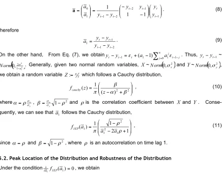
since . Now ~ , therefore ~ . From Eq. (6), we can obtain the

. (8)

therefore

. (9)

On the other hand, From Eq. (7), we obtain . Thus, ~

. Generally, given two normal random variables, ~ and ~ ,

we obtain a random variable which follows a Cauchy distribution,

, (10)

where , and is the correlation coefficient between and .

Conse-quently, we can see that follows the Cauchy distribution,

, (11)

since and , where is an autocorrelation on time lag 1.

5.2.Peak Location of the Distribution and Robustness of the Distribution

Under the condition , we obtain

. (12)

Figure 4 shows autocorrelations of on the time lag 1, , for given AR(1) parameter

, where . Note that does not depend on the value of .

This graph shows that the location of the peak of , , is always negative although the

given AR(1) parameter .

It is known that power law distributions generated by some nonlinear systems are fragile for pa-rameter change (Kamiura and Gunji 2006). By contrast, the distribution (11), which shows power law in the tail, is robust for the parameter change : i.e. If , then we obtain

and ~ , thus follows the distribution (11).

5.3.Computational Experiments

We can computationally confirm the analyses in the previous sections. Assume an AR(1),

, (13)

where ~ and .

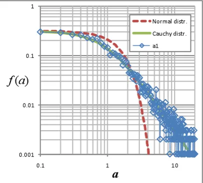
Figure 5(a) and Figure 5(b) show a distribution of IEP given by Eq. (9), a normal distribution

( , ) and a Cauchy distribution given by Eq. (10)

( , ). Figure 5(b) is double logarithmic graphs.

Figure 5(a): The graphs of a distribution of , a normal distribution ( , ) and a

Figure 5(b): The double logarithmic graphs of a distribution of , a normal distribution

( , ) and a Cauchy distribution ( , ).

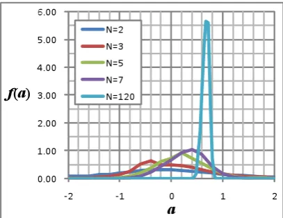
Figure 6 shows asymptotic property of the distribution of defined by Eq. (5). The distributions of get closer to a normal distribution with , as N gets larger. In this process, the power law property of the Cauchy distribution in Figure 5 vanishes away. In N = 120, we can see conventional

parameter estimation, in which follows a normal distribution with and

.

Figure 6: The asymptotic property of the distribution of .

6.

Conclusion

Abduction is a kind of logical inference, and has been studied not only in philosophy (Peirce 1868; 1955) but also in artificial intelligence and computer science (Bylander et al 1991; Tanner and Jo-sephson 1996; Finlay and Dix, 1996; Abe 2003).

In this paper, we integrate Finlay-Dix's representation of abduction (1996) and Sawa-Gunji's one (2010). Integrated representation derives a numerical aspect of abduction, which is identified as incomplete parameter estimation. We introduce the incompleteness for parameter estimation of AR(1) process.

As a result of the numerical analyses, the IEP follows a Cauchy distribution, which has a power law of the slop -2 in the tail, although conventionally estimated parameter is normally distributed. The Cauchy distribution is caused by a ratio distribution of normal random variables which is gen-erated from the AR(1) process.

References

Awodey, S. (2006). Category Theory. Oxford: Oxford University Press.

Abe, A. (2003). The Role of Abduction in Chance Discovery. New Generation Computing 21(1), 66-71.

Bak, P., Tang, C., & Wiesenfeld, K. (1987). Self-organized criticality: An explanation of the 1/f noise. Phys. Rev. Lett., 59, 381-384.

Bylander, T., Allemang, D., Tanner M.C. & Josephson, J.R. (1991). The computational complexity of abduction. Artificial Intelligence, 49, 25-60.

Claycomb, J.R., Nawarathna, D., Vajrala. V., & Miller, J.H. (2004). Power law behavior in chemical reactions. J. Chem. Phys., 121(24), 12428-12430.

Finlay, J. & Dix, A. (1996). An Introduction to Artificial Intelligence. London: UCL Press.

Gunji Y.-P. & Kamiura M. (2004). Observational heterarchy enhancing active coupling. Physica D, 198, 74-105.

Kamiura, M. & Gunji,Y-P. (2006). Robust and Ubiquitous On-Off Intermittency in Active Coupling. Physica D, 218, 122-130. Kamiura, M. (2010). Implication of Abduction: Complexity Without Organized Interaction. Proceedings of the 9th _{International}

Conference on Computing Anticipatory Systems, accepted.

Luque, B., Miramontes, O. & Lacasa, L. (2008). Number theoretic example of scale-free topology inducing self-organized criticality. Phys. Rev. Lett., 101, 158702.

MacLane, S. (1971). Categories for Working Mathematician. New York: Springer, 1997 (2nd ed.). Marsaglia, G. (2006). Ratios of normal variables. Journal of Statistical Software, 16(4).

Peirce, C.S. (1868). Some Consequences of Four Incapacities, In: Charles Hartshorne and Paul Weiss, Collected papers of Charls Sanders Peirce. Harvard: Harvard University Press, 1960.

Peirce, C.S. (1955). Abduction and Induction. In: Philosophical Writings of Peirce (Chapter 11), Dover Publications. Sawa, K. & Gunji, Y-P. (2010). Dynamical Logic Driven by Classified Inferences Including Abduction. Conference

Proceed-ings of the 9th _{International Conference on Computing Anticipatory Systems, accepted.}

Tanner, M.C. & Josephson, J.R. (1996). Conceptual analysis of abduction. In: J.R. Josephson and S.G. Josephson(Ed.),

Abductive Inference: Computation, Philosophy, Technology (Chapter 1). Cambridge: Cambridge University Press.

About the Author

Moto Kamiura

March 2007: Doctor of Science on Physics, Kobe University June 2007 - March 2008 Technical Assistant in Kobe University