From here and now to there and then : practical recommendations for extrapolating cetacean density surface models to novel conditions

Technical report 2019-01

From here and now to there and then:

Practical recommendations for

extrapolating cetacean density surface

models to novel conditions

Phil J. Bouchet, Dave L. Miller, Jason J. Roberts, Laura Mannocci, Catriona M. Harris, Len Thomas

From here and now to there and then:

Practical recommendations for

extrapolating cetacean density surface

models to novel conditions

Phil J. Bouchet § _{, Dave L. Miller} § _{, Jason J. Roberts} ¶ _,

Laura Mannocci ¶, ☨ _{, Catriona M. Harris} § _{, Len Thomas} §

§ _{Centre for Research into Ecological & Environmental Modelling, School of Mathematics and Statistics,}

University of St Andrews, Scotland

¶ _{Marine Geospatial Ecology Lab, Duke University, Durham, United States}

☨ _{MARBEC (Marine Biodiversity, Exploitation and Conservation), University of Montpellier, CNRS, Ifremer,}

IRD, Sète, France

Document control

Report code CREEM-2019-01

Date 15 August 2019

Rev. Date. Reason for Issue Prepared by Checked by

1 2019-05-01 Sent to DM for internal review PB DM 2 2019-06-03 Sent to project team for final review PB, DM Team

Please cite this report as:

Enquiries should be addressed to

Prof. Len Thomas | [email protected] Dr. David L. Miller | [email protected] Dr. Phil J. Bouchet | [email protected]

Centre for Research into Ecological & Environmental Modelling (CREEM)

The Observatory, Buchanan Gardens, University of St Andrews, St Andrews Fife, KY16 9LZ, Scotland (UK)

Copyright

This report is licensed for use under a Creative Commons Attribution 4.0 Licence. For licence conditions, see

https://creativecommons.org/licenses/by/4.0/

Acknowledgements

This work forms an output from the DenMod project (Working group for the advancement of marine species density surface modelling ) and was supported through funding by the United 1 States Office of Naval Research (ONR) under the Living Marine Resources (LMR) programme . 2 PJB, DLM, JJR, CLH, and LT were funded by OPNAV N45 and the SURTASS LFA Settlement Agreement, managed by the U.S. Navy's Living Marine Resources programme under Contract No. N39430-17-C-1982.

Table of contents

List of figures 4

List of tables 4

Acronyms 5

Executive summary 6

1. Introduction 7

1.1 Scope 8

1.2 Objectives 9

2. A short review of extrapolation in environmental space 12

2.1 Definition 12

2.2 Why extrapolate? 15

2.3 Error sources and assumptions 18

2.4 Some solutions 24

2.5 Extrapolation metrics 26

3. Software 33

4. Outlook and recommendations 34

5. Future directions 38

List of figures

Figure 1. Map of cetacean line transect surveys conducted in the Northwest Atlantic and Gulf of Mexico.

Figure 2. Basic types of extrapolation used in ecology.

Figure 3. Schematic representation of extrapolation in the environmental space defined by two hypothetical biotic/abiotic covariates relevant to humpback whales.

Figure 4. Example of errant extrapolation in the estimation of North Atlantic right whale size as a function of age.

Figure 5. Real-world example of errant extrapolation in a density surface model of beaked whales.

Figure 6. Effects of upscaling a bathymetric grid of the U.S. Navy’s Atlantic Fleet Training and Testing (AFTT) area, in the Northwest Atlantic.

Figure 7. Three approaches to dealing with extrapolation in predictive ecological models.

Figure 8. Typology of environmental extrapolation.

Figure 9. Conceptual representation of two key extrapolation metrics.

Figure 10. Simple matrix for interpreting extrapolation assessments based on the combination of ExDet and %N.

List of tables

Table 1. Common sources of errors encountered in ecological extrapolation.

Table 2. Summary of the main extrapolation diagnostics used in ecological models. 12

14

27 24 21 16 15

30

31

37

19

Acronyms

AFTT Atlantic Fleet Training and Testing (area)

CBD Convention on Biological Diversity

DSM Density Surface Model

EBV Essential Biodiversity Variable

EEZ Exclusive Economic Zone

ESA Endangered Species Act

GAM Generalised Additive Model

GEO BON Group on Earth Observations Biodiversity Observation Network

IUCN International Union for the Conservation of Nature

LMR Living Marine Resources

MMPA Marine Mammal Protection Act

NAEMO Navy Acoustic Effects Model

Executive summary

Density surface models (DSMs) are clearly established as a method of choice for the analysis of cetacean line transect survey data, and are increasingly used to inform risk assessments in remote marine areas subject to rising anthropogenic impacts (e.g. the high seas). However, despite persistent skepticism about the validity of extrapolated models, more and more DSMs are being applied well beyond the boundaries of the study regions where field sampling originally took place. This leads to potentially uncertain and error-prone model predictions that may mislead on-the-ground management interventions and undermine conservation decision-making. In addition, no consensus currently exists on the best way to define and measure extrapolation when it occurs, leaving users without the tools they require to audit models projected into novel conditions. Consequently, a transparent and consistent protocol for identifying scenarios under which extrapolation may be appropriate (or conversely, ill-advised) is urgently needed to better gauge how models behave outside the boundaries of sample data and to know how much faith can be placed in their outputs.

This report aims to address this gap by synthesising recent advances in extrapolation detection, and presenting recommendations for a minimum standard for measuring extrapolation in novel environmental space. Such guidelines are essential to promoting transparency, replicability, and quality control, and will help marine scientists, managers and policy agencies to (i) better interpret density surfaces and their associated uncertainty; (ii) refine model development and selection approaches; and (iii) optimise the allocation of future survey effort by identifying priority knowledge gaps, e.g. by delineating areas where model predictions are the least supported by data. Our review is accompanied by supplementary R code offering a user-friendly framework for quantifying, summarising and visualising various forms of extrapolation in multivariate environmental space a priori (ahead of model fitting). We illustrate its application with case studies designed to revisit previously published predictions of sperm whale ( Physeter macrocephalus ) and beaked whale ( Ziphiidae spp. ) densities in the Northwest Atlantic, and evaluate them in light of several extrapolation metrics.

1. Introduction

The expanding footprint of human activities across the world’s oceans is rapidly creating novel challenges for the conservation of marine vertebrate populations globally (Lewison et al. 2014; Halpern et al. 2015) . With more than a quarter of all extant cetacean species (i.e. whales and dolphins) currently believed to face extinction (Davidson et al. 2012) , geographically-explicit risk assessments are urgently required to mitigate the cumulative impacts of anthropogenic threats such as fisheries bycatch, noise pollution, and climate change, amongst numerous others (Avila et al. 2018) . Reliable estimates of cetacean abundance or density patterns in both space and time are fundamental to addressing this need, but remain difficult to obtain in many marine areas subject to limited sampling effort (e.g. the high seas; Kaschner et al. 2012) .

In this context, the development of predictive statistical models that can estimate cetacean abundance as a function of spatially- and temporally-referenced environmental covariates – both static (e.g. seabed depth and slope) and dynamic (e.g. sea surface temperature, primary productivity) – has greatly accelerated over the last decade (Guisan & Zimmermann 2000; Guisan & Thuiller 2005; Redfern et al. 2006; Ready et al. 2010; Dambach & Rödder 2011; Robinson et al. 2011, 2017; Marshall et al. 2014) . In particular, GAM -based density surface 3 models (Hedley & Buckland 2004; hereafter DSMs; Miller et al. 2013) are now clearly 4 established as a method of choice for the analysis of cetacean line transect surveys in the presence of imperfect detectability, and provide useful tools for generating policy-relevant knowledge in support of applied management against a backdrop of data deficiency (Becker et al. 2012; Hammond et al. 2013; Redfern et al. 2017; Derville et al. 2018) . For instance, DSM outputs have recently been used to guide the designation of marine protected areas (e.g. Cañadas & Vázquez 2014) , inform the rerouting of major shipping lanes (e.g. Redfern et al. 2013) , assist the planning of military exercises (e.g. Mannocci et al. 2017b) , or forecast cetacean population dynamics in the face of extreme weather events (Becker et al. 2018) .

Immediate and pressing demands for solutions to large-scale management problems are increasingly encouraging the application of ecological models well beyond the boundaries of the study regions where sampling originally took place (Miller et al. 2004; Sequeira et al. 2018a) , such that many cetacean DSMs involve some degree of extrapolation (e.g. Mannocci et al. 2015; Virgili et al. 2018; García-Barón et al. 2019) . Very early in their training, scientists are warned against extrapolating (Conn et al. 2015a) , as inference outside the range of the sample relies on fundamental assumptions that lack direct empirical support from the available data (Elith & Leathwick 2009; Escobar et al. 2018; Qiao et al. 2019) and may lead to extreme predictions with only limited biological realism (Owens et al. 2013) . Accordingly, most models

3 _{GAM: Generalised additive models (see Wood 2017 for technical details) .}

4 _{Two or more stage modelling framework combining a spatial model of abundance with a detection}

transferred into novel temporal and/or spatial domains are expected to be fraught with both statistical and ecological errors (Clark et al. 2001; Peters & Herrick 2004) , the magnitude of which can vary substantially across taxonomic groups, habitats, and/or modelling algorithms (e.g. Fielding & Haworth 1995; Shabani et al. 2016; Redfern et al. 2017) . It is unsurprising, therefore, that appropriate evaluations of model prediction uncertainty and extrapolative capacity under previously un-encountered environmental scenarios are rapidly emerging as an active and important area of research in applied ecology and conservation (Steen et al. 2017; Yates et al. 2018) .

1.1 Scope

As acoustically-specialised animals, cetaceans are sensitive to the negative effects of chronic and acute exposure to man-made underwater noise (Williams et al. 2015) . For instance, the noise generated as a by-product of commercial maritime traffic or seismic exploration can mask species’ acoustic communication signals, disrupt diving behaviour, elicit physiological stress, and/or cause displacements from favoured habitats, ultimately interfering with key life functions such as foraging, mating, nursing, and/or resting (Tyack 2008; Erbe et al. 2018; Gordon 2018; Wensveen et al. 2019) . Intense impulsive sounds from high-power mid-frequency naval sonar have also been linked with atypical mass stranding events in several species (Jepson et al. 2003; D’Amico et al. 2009; Filadelfo et al. 2009) and are thus of serious concern, although available evidence from controlled exposure experiments suggests that measurable behavioural responses may vary between and within individuals and populations (e.g. DeRuiter et al. 2013; Goldbogen et al. 2013; Southall et al. 2016; Harris et al. 2018) . In recognition of anthropogenic underwater noise as a world-wide problem, a rising number of calls are being made to strengthen management and mitigation frameworks for sound-producing activities (Dolman & Jasny 2015) .

these locations have not been surveyed for marine mammals, then density estimates are usually obtained from DSMs extrapolated from adjacent sampled areas.

1.2 Objectives

A transparent and uniform approach to quantifying extrapolation is a critical prerequisite to furthering our understanding of how models may behave outside the bounds of the data from which they are built (Escobar et al. 2018) , and therefore to knowing how much credence or skepticism their outputs should be given. Although several extrapolation metrics have already been proposed in the peer-reviewed literature (e.g. Elith et al. 2010; Rödder & Engler 2012; Zurell et al. 2012; Mesgaran et al. 2014; Conn et al. 2015a) , little consensus exists on which proves most appropriate for a given dataset, with limited clarity on how extrapolation affects predictions generated by models developed from different types of data (e.g. abundance vs. presence-only data). In particular, general rules for supporting consistent assessments of extrapolation remain lacking in cetacean studies, prompting an urgent need to standardise best practice in model evaluation (Sequeira et al. 2018a) .

The purpose of this report is to propose a series of practical guidelines for diagnosing, measuring, and visualising extrapolation in novel multivariate environmental space. While our primary focus is on density surface models of cetacean populations, the general concepts and software tools presented herein are equally relevant to other types of models, and applicable to other taxa or other forms of biological data. Note that we concentrate on extrapolation as defined by Strong & Elliott (2017) , i.e. the estimation of a response function (empirical or mechanistic), that allows predictions of an ecological variable to be obtained based on a set of observations and a number of predictor (explanatory) covariates. Other approaches to ecological scaling do exist (e.g. lumping) but are not dealt with here (see Strong & Elliott 2017 for details) . Furthermore, given inherent variability in the predictive performance of different model algorithms (Meynard & Quinn 2007; Rapacciuolo et al. 2012; Beaumont et al. 2016; Yates et al. 2018) , we only consider extrapolation assessments performed a priori , i.e. before model fitting. As such, the extrapolation detection approaches described below can only be used to identify potential areas where model predictions may be prone to errors. The magnitude of these errors, or their associated uncertainty, is however likely to differ between model types and parameterisations. Notwithstanding, we expect that standard guidelines for quantifying extrapolation will assist marine scientists, managers and policy agencies in:

● Better interpreting model predictions (e.g. density surfaces) and their associated uncertainty;

● Refining model development and selection protocols accordingly;

The report is structured as follows:

● The next section contains an overview of extrapolation in novel environmental space. In it, we define and illustrate various extrapolation scenarios, explain why extrapolating is critical (and inevitable) in many cetacean studies, and succinctly review the range of extrapolation diagnostics currently available, highlighting two that are of particular value for use with DSMs. In addition, we list the key assumptions made when projecting models into novel conditions to improve awareness of the potential pitfalls associated with extrapolation.

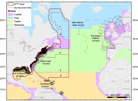
● Following from this, we briefly describe a set of custom functions developed in the programming language R ( https://cran.r-project.org/ ) to assist extrapolation assessments in DSMs and other predictive models. We provide links to the code, which draws upon real-world abundance data from line transect surveys of cetaceans undertaken aboard shipboard and airborne sampling platforms across portions of the U.S. and Canada’s Exclusive Economic Zones (EEZ) (equivalent to ca. 1.1 million linear km of total effort; Fig. 1 ). Survey details and data sources are fully described in Roberts et al. (2016) and Mannocci et al. (2017b) .

Figure 1 : Map of cetacean line transect surveys conducted in the North Atlantic basin (including the U.S. EEZ and Gulf of Mexico). The U.S. Navy Atlantic Fleet Training and Testing (AFTT) area (which excludes territorial waters <12 nautical miles of the shore) is shown as a red outline (11 x 10 6 _km 2 _{). Line transect}

2. A short review of extrapolation in environmental space

2.1 Definition

To extrapolate means:

‘ To project or expand existing knowledge in order to generate insights about an unknown system, based on an assumed continuity, correspondence, or other parallelism between it and the observed data. ’ (Miller et al. 2004) .

Put simply, extrapolating is the act of using a point/region of reference , where baseline 5 information exists, to estimate the value(s) of a variable at another target point/region, which 6 has not been sampled and for which predictions are sought (Munns 2002) .

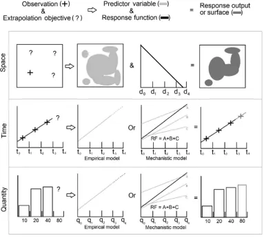
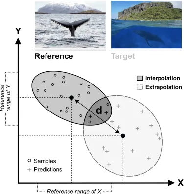
In ecology, extrapolation is typically performed over space (e.g. between regions differing in latitude and longitude), and/or over time (e.g. into the future or the past), although alternative forms of extrapolation are also commonplace in related disciplines ( Fig. 2 ) (e.g. across taxonomic levels or ontogenetic stages in experimental biology and laboratory studies; amongst doses and exposure regimes in ecotoxicology) (Solomon et al. 2008) . The magnitude (extent) of extrapolation can be conceptualised as a dissimilarity index (or distance) between target and reference systems ( Fig. 3 ) in the multivariate space defined by their respective environmental conditions (Radeloff et al. 2015; Sequeira et al. 2018a) . The greater this distance, the stronger the extrapolation. Note that, in this case, extrapolation is measured along the chosen environmental dimensions of interest, rather than in geographic (e.g. in km, using Cartesian coordinates) or temporal (e.g. hours, days, weeks) space (Booker & Whitehead 2018) . This means that some extrapolations may fail immediately after the reference domain is abandoned (eg. in adjacent areas; Osborne & Foody 2007) , or conversely, that others made across continents/ocean basins or through centuries are theoretically permissible so long as reference and target conditions are sufficiently similar (Yates et al. 2018) .

Extrapolation is problematic for a multitude of reasons (see section 2.3 ), and a growing body of literature now documents how ecological inference becomes perilous outside the scope of the data used for model training (Graf et al. 2006; Dormann 2007; Fisher & Naidoo 2011; Torres et al. 2015; Bell & Schlaepfer 2016; Péron et al. 2018) . Part of the danger stems from the fact that even models that adhere closely to sample observations can yield misleading outputs if they fail to capture the underlying process that generated the data in the first place (Heikkinen et al. 2012) . This is perhaps best understood in the context of a simple univariate regression analysis.

5 _{Also referred to as ‘source’, ‘training’, ‘internal’ or ‘calibration’ system/domain.}

Figure 2 : Basic types of extrapolation. Spatial and temporal extrapolations (top and middle) are common in ecology, and are the focus of the present report. Figure reproduced from Strong & Elliott (2017) with permission from Elsevier.

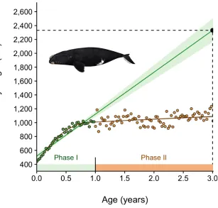
Figure 4 : Example of errant extrapolation in the estimation of North Atlantic right whale ( Eubalaena glacialis ) size as a function of age. The species exhibits differential growth rates at various stages of maturity, with calves gaining considerable mass while nursing (a daily average of ∼1.7 cm and ∼34 kg

during the first twelve months of life; Phase I), and growing much more slowly thereafter (Phase II). Despite an excellent fit (adjusted R 2 _{= 0.89), a simple linear model fitted to Phase I data only ignores the}

asymptotic nature of growth and substantially overpredicts the body length of mature individuals (e.g. 23.3 m at 3 years of age, 95% CI 21.6 - 25 m, i.e. larger than some subspecies of blue whales). Data from Fortune et al. (2012) . Right whale silhouette credits: NOAA Fisheries ( https://www.fisheries.noaa.gov/ ).

2.2 Why extrapolate?

Extrapolation has two primary motivations in ecological research.

2017) . Knowledge gaps are most prevalent in marine systems, especially in the deep pelagic ocean (Webb et al. 2010; Kaschner et al. 2012; Bouchet 2015) , which is remote and inaccessible, and across the EEZs of many developing countries (Jarić et al. 2014) , where financial resources are insufficient for even basic information on species occurrence to be gathered (Braulik et al. 2018) . Such levels of data deficiency pose a serious roadblock to furthering progress towards meeting the Convention on Biological Diversity’s (CBD) Aichi Targets, as they compromise estimates of extinction risk and lead to many little known organisms being overlooked in conservation planning (Bland et al. 2015; Walls & Dulvy 2019) . In many situations where data simply do not exist, extrapolation therefore represents a practical inevitability, and an essential component of criteria setting in ecological risk assessments. Unsurprisingly, the use of extrapolative models has experienced explosive growth in recent decades, particularly by governmental and non-governmental organisations charged with natural resource and endangered species management at large spatial scales (Franklin 2010a) .

et al. 2009) . In the global ocean, an inherently dynamic environment subject to planet-level changes, forecasting without extrapolation may therefore be altogether unfeasible (Berteaux et al. 2006) .

In the face of unabated marine and terrestrial defaunation crises (Dirzo et al. 2014; McCauley et al. 2015) , enormous challenges remain for even simply assessing progress towards meeting the CBD’s Aichi Targets, particularly on a global scale (Kissling et al. 2018) . As a result, the concept of essential biodiversity variables (EBVs) was proposed by the Group on Earth Observations Biodiversity Observation Network (GEO BON) in 2013 as a harmonised system for delivering aggregated data on major dimensions of biodiversity loss and change (Pereira et al. 2013; Schmeller et al. 2017) . Population abundance is one of 22 such EBVs (Kissling et al. 2018) and is a useful metric that can underpin assessments of extinction risk for threat categorization (Butchart et al. 2010) , and serve as an early signal of the relative severity of expected impacts to ecosystems (Kulhanek et al. 2011) . However, despite its obvious value to policy and decision-making (e.g. Acevedo et al. 2014) , knowledge of population abundance remains scant for the majority of species (Bowler et al. 2019) . This is in great part due to the difficulties of making accurate counts of organisms in the field, compared to simply recording their presence. As a consequence, abundance models usually entail a significant amount of spatial and temporal extrapolation, and remain more challenging to fit for many (marine) taxa (Sequeira et al. 2018b) . That said, the superior information content associated with abundance data is expected to enhance transferability, so that extrapolated models of abundance, when available, might be better projected into non-analogue conditions than say, presence-absence models (Howard et al. 2014) .

Many marine mammals, including cetaceans, are wide-ranging, highly mobile, cryptic, rare, and thus hard to survey, such that ca. 40% of extant species are currently inadequately known (Schipper et al. 2008) . More than a third (36%) are also long-distance migrants with specialised diets that undertake ocean basin-scale movements to exploit seasonally available habitats and resources in multiple locations (Robinson et al. 2009) . Ecological risk assessments for such data-poor ‘moving targets’ can seldom proceed without applying previously established ecological relationships to new areas, scales, and/or time periods (Clark et al. 2001) , and extrapolation has therefore become commonplace in cetacean studies (Mannocci et al. 2015, 2017b; Roberts et al. 2016; Redfern et al. 2017) , particularly where inference about broad-scale species distribution and abundance patterns is required to support on-the-ground management (Strong & Elliott 2017) .

2.3 Error sources and assumptions

Thomas 1975; Riegelman 1979; Xiao & Yung 2015) , and are covered in nearly every introductory statistics textbook (Zar 1999; Gillman 2009; Guisan et al. 2017) . A telltale example of nonsensical extrapolation was provided in the early 1870s by Mark Twain:

“ In the space of one hundred and seventy-six years, the Lower Mississippi has shortened itself two hundred and forty-two miles. That is an average of a trifle over one mile and a third per year. Therefore, any person [...] can see that [...] a million years ago, the Lower Mississippi River was upward of one million three hundred thousand miles long, and stuck out over the Gulf of Mexico like a fishing rod. By the same token, any person can see that seven hundred and forty-two years from now, the lower Mississippi will be only a mile and three-quarters long, and Cairo and New Orleans will have joined their streets together, plodding comfortably along under a single mayor with a mutual board of aldermen. ”

Likewise, Von Foerster et al. (1960) ’s tongue-in-cheek prediction that the world’s human population would reach infinite size on November 13, 2026 - i.e. ‘Doomsday’ - was based on an extrapolation of growth models fitted to historical data. Clearly, extrapolations are sensitive and prone to a number of errors that may bias model outputs, impair prediction accuracy, and inflate uncertainty (Dormann 2007; Oliver & Roy 2015; Qiao et al. 2019) ( Table 1 ).

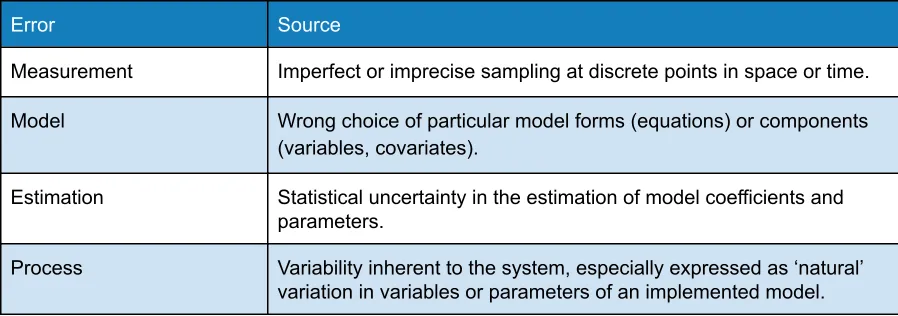
Table 1 : Common sources of errors encountered in ecological extrapolation. Modified from Peters and Herrick (2004) .

Error Source

Measurement Imperfect or imprecise sampling at discrete points in space or time. Model Wrong choice of particular model forms (equations) or components

(variables, covariates).

Estimation Statistical uncertainty in the estimation of model coefficients and parameters.

Process Variability inherent to the system, especially expressed as ‘natural’ variation in variables or parameters of an implemented model.

Although the magnitude of errors is likely to vary amongst taxa, ecosystems, and/or modelling scenarios, most errors largely stem from violations of a number of key underlying assumptions (Richmond et al. 2010; Jarnevich et al. 2015; Guisan et al. 2017) , including:

expanding into habitats that have only recently become available, or if the regional population is insufficient to support colonisation (Wiens et al. 2009) . Other factors such as group living and sociality, learning and memory processes, age or reproductive status-mediated habitat selection, migratory movements, dispersal lags or barriers, and biotic interactions (e.g. competition, predator avoidance, or pathogens) may also prevent individuals from accessing, or persisting in, suitable sites (Channell & Lomolino 2000; Svenning & Skov 2004; Václavík & Meentemeyer 2012) . For instance, West Australian bottlenose dolphins ( Tursiops aduncus ) have been shown to remain in less prey-rich, but safer, shallow habitats during periods of high shark abundance (Heithaus & Dill 2006) . Conversely, breeding-area philopatry and overcrowding in high-density populations may restrict some individuals to suboptimal conditions. Models developed in non-equilibrium settings (e.g. invasions, climate change) may thus involve biased records that are unrepresentative of species’ habitat requirements and may lead to unreliable predictions (Elith & Leathwick 2009; Jachowski et al. 2016) . Although this is an important assumption for transferring models in space or time, there have been surprisingly few critical appraisals of how close a given modelled system really is to equilibrium, or how long it would take to reach a new state of equilibrium, e.g. after environmental change (Guisan et al. 2017) .

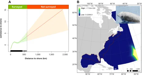
● Adequate sampling: Extrapolations are more likely to be spurious if samples themselves fail to encompass the full range of relevant environmental gradients present in the reference and target systems (Braunisch & Suchant 2010) ( Fig. 5 ). Sampling effort varies across the globe, with much higher survey intensity in the vicinity of populated areas and in temperate regions (Anderson 2012) . It is also common for ecologists to delineate their study areas arbitrarily according to geopolitical borders or other practical boundaries (El-Gabbas & Dormann 2018) . Consequently, many biological datasets prove incomplete or exhibit spatial bias (e.g. Corkeron et al. 2011) , resulting in models with truncated response curves that may under-represent areas of suitable habitats and suffer from limited predictive power (Vaughan & Ormerod 2003; Thuiller et al. 2004; Powers et al. 2011; Sánchez-Fernández et al. 2011) .

niches are more similar to one another than to any random niche fitted in the same realised environment) can signal potential issues, but the former is usually so strict that it rejects niche overlap for most species, and the latter too liberal, such that even minute amounts of niche overlap will suffice for reference and target systems to be declared comparable (Guisan et al. 2017) . A pragmatic yet data-intensive solution is to quantify the relationship between model extrapolation success and niche overlap. Where data availability allows such assessments, it is possible to use simple estimates of niche overlap as indicators of whether a model is likely to project well to a different area or time period (Guisan et al. 2017) .

● Appropriate covariate choice: The selection of adequate explanatory covariates is a prominent issue in predictive modelling (Wiens et al. 2009) , which hinges not only on data availability but also on an understanding of the underlying mechanisms responsible for observed species’ distribution and abundance patterns (Petitpierre et al. 2017; Fourcade et al. 2018) . For instance, a frequent misconception is that species are exclusively affected by physical habitat features, when in fact their current distributions may also reflect historical human disturbance and landscape use (Fois et al. 2018) . Extrapolations are likely to be particularly error-prone if distal (i.e. indirect) covariates are used, as correlations between these and true proximal drivers may fluctuate both spatially and temporally (Austin 2002; Yates et al. 2018) . This may be exacerbated by measurement errors in covariate layers, an issue that has received limited attention in the predictive modelling literature (Guisan et al. 2017) . Overall, important covariates that are unavailable should be identified a priori , and implications for model predictions anticipated (and discussed) to avoid drawing spurious conclusions (Guisan et al. 2017) .

● Stationarity: For extrapolation to work, species-habitat relationships must be consistent and comparable in shape, direction, and amplitude within both the reference and target systems (the concept of “transportability”; Vaughan & Ormerod 2005) . This implies that heterogeneity in both habitat availability and habitat selection between individual animals is deemed negligible (Osborne & Suárez-Seoane 2002) , which is seldom reasonable. The assumption of stationarity also rarely holds for processes operating over large geographic areas or at fine resolutions (Unwin & Unwin 1998) . With growing appetite for extrapolating models on global scales, there is a risk of including areas where animals respond to habitats in different ways (e.g. due to social status) (Osborne & Suárez-Seoane 2002) .

● Adaptability: Extrapolation assumes immediate adaptations to novel conditions, and while rapid evolutionary change is possible (Thompson 1998; Franks et al. 2007; Koch et al. 2014) , it has only been empirically demonstrated in a few short-generation species. If species display high genetic, behavioural or phenotypic plasticity, extrapolation outputs may well be more variable (e.g. large predicted range) than under the assumption of genetic and phenotypic constancy (Rehfeldt et al. 2001) .

● Space-for-time substitutability: Because long-term ecological time-series are generally rare, a common approach to performing temporal extrapolations is to develop models across multiple contemporary sites whose current conditions mimic the range of those known to have occurred in the past, or anticipated to arise in the future (Lester et al. 2014) . The relationships identified across these spatial gradients are then used as surrogates for predicting temporal processes. Although successful in a number of cases (Banet & Trexler 2013; Blois et al. 2013a; Rolo et al. 2016) , this approach could pose problems in non-stationary environments where the drivers of spatial and temporal turnover differ and where some of the key factors controlling population dynamics may remain unobserved but vary spatially (Damgaard 2019) .

It is essential to understand the above assumptions, as failing to meet them can lead to both errors of omission (false negatives) and errors of commission (false positives) (Richmond et al. 2010; Sohn et al. 2013) that will undermine model interpretation. As an example, commission errors will lead to overestimations of species’ range expansions in climate change studies, whereas omission errors will make range contractions appear more severe than they actually are (Rangel & Loyola 2012) . Extrapolated models are particularly susceptible to the former, because the data used for model parameterisation seldom encompass the entire range of conditions present in the target region (Carneiro et al. 2016) . Furthermore, extrapolation is risky in situations where response curves are high or increasing at the edges of the calibration domain ( Fig. 5 ) (Peterson et al. 2011) , and including descriptive spatial structures (e.g. via conditionally autoregressive models) can lead to misleading predictions of abundance around the edges of study areas (i.e. edge effects) or where there are large gaps in survey coverage (Ver Hoef & Jansen 2007; Conn et al. 2014, 2015b) .

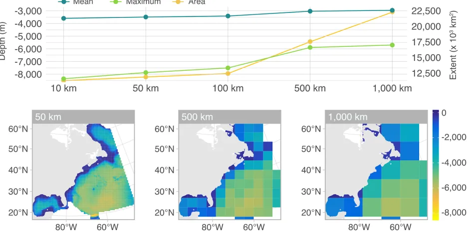
At coarser grains, the span of explanatory covariates decreases dramatically, such that two maps produced at different resolutions also exhibit different geographic extents and value ranges (Guisan et al. 2017) ( Fig. 6 ). As a result, extrapolation errors are likely to arise when projecting a model fitted at a coarse grain to a finer grain (Randin et al. 2009) . Hierarchical Bayesian frameworks offer one way of alleviating extrapolation issues associated with changes in grain size, e.g. by considering abundance at fine resolution as a latent variable that can be modelled as a function of fine-scale environmental covariates and constrained by observed abundances at coarser scales (see Keil et al. 2013 for an example) .

Figure 6 : Effects of upscaling a bathymetric grid of the U.S. Navy’s Atlantic Fleet Training and Testing (AFTT) area, in the Northwest Atlantic. The top panel shows the mean and maximum depth as well as the surface area for rasters at different resolutions. The bottom panel shows three example maps. The range of depth values shrinks when the original raster, available at 10 km resolution, is resampled to coarser grains (50, 100, 500, and 1000 km).

contemporaneous to animal presence, abundance or movement (e.g. daily, weekly), versus averaged products (monthly, seasonal, climatological) all the more crucial (Scales et al. 2017) .

Ultimately, no single model can be expected to work flawlessly for all taxa, in all areas, and at all times (Jarnevich et al. 2015; Qiao et al. 2015) . It is worth noting, therefore, that extrapolation is also influenced by model choice, model complexity, and model tuning (Buisson et al. 2010; Anderson & Gonzalez 2011; Merow et al. 2014) . Numerous studies have attempted to benchmark the performance of different modelling approaches under a range of parameterisation scenarios, with mostly inconsistent results (Meynard & Quinn 2007; Syphard & Franklin 2009; Beaumont et al. 2016; Shabani et al. 2016) . A practical dilemma is that several model structures or formulations may fit the reference data equally well (an issue known as ‘equifinality’ or ‘non-identifiability’) (Bucklin et al. 2015) , yet lead to diverging predictions in the target system (Fygenson 2008; Dormann et al. 2012; Domisch et al. 2013) . Simpler, more parsimonious models are often preferred to maximise ecological realism and interpretability. However, they also threaten to ignore key processes and, with insufficient flexibility to describe ecological relationships, can extrapolate poorly (Thuiller et al. 2004; Evans et al. 2013) . By contrast, extrapolation is naturally more pervasive when the number of covariates increases (Authier et al. 2017) , and more complex and flexible models risk overfitting - i.e. capturing data idiosyncrasies and noise at the expense of true signals - such that they will not generalise to conditions other than those encountered during calibration (Bell & Schlaepfer 2016) . While this has led some authors to advocate for models of intermediate complexity (Moreno-Amat et al. 2015) , building simple and complex models may ultimately serve different purposes, and a preference for one approach over another may be equally justifiable depending on the specific context of a given study (see Merow et al. 2014 for a detailed discussion) . For example, an ‘overfitting’ model may be more desirable for identifying areas suitable for the re-introduction of rare captive-bred species, whereas simpler models may be better equipped to guide searches for remnant populations of possibly extinct species (Escobar et al. 2018) . In any case, it is clear that predictions from correlative models are often only as good as our knowledge of the mechanisms and feedbacks that underlie ecological patterns (Miller et al. 2004) . Successful models are therefore likely to be those based on relatively simple relationships grounded in mechanisms that are well understood (Yates et al. 2018; Bouchet et al. 2019) .

2.4 Some solutions

questions relating to non-analogue climate scenarios or species’ range expansions (Merow et al. 2014) .

Three main strategies have therefore been proposed to deal with extrapolation (but see Elith & Leathwick 2009 for additional solutions) , namely: avoidance, mitigation, and diagnosis (Owens et al. 2013; Sequeira et al. 2018a) .

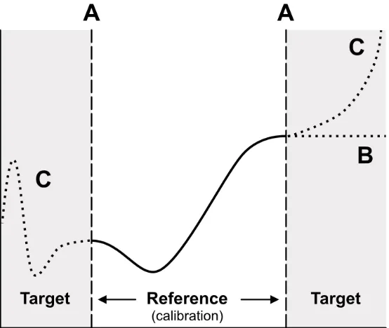
● Avoidance: Truncating model predictions ( Fig. 7 A ) by discarding or masking any that are produced outside the space of the reference data offers a simple and effective way of avoiding extrapolation. There have been suggestions that extrapolations may be deemed negligible if model predictions are not made beyond one-tenth of the sampled covariate range (Dormann 2007) . However, this is only a generic guideline that is unlikely to provide consistent results in most contexts.

● Mitigation: Clamping (or ‘bounding’), i.e. holding predictions constant at the marginal value obtained in the calibration area ( Fig. 7 B ), can help alleviate potential extrapolation errors and is the default setting in some software packages such as MaxEnt (Stohlgren et al. 2011; Merow et al. 2013) . Although this is a conservative approach, clamping at high values may lead to density estimates that are inflated unrealistically when extrapolating (Guevara et al. 2018) . A more pragmatic solution would be to reduce the likelihood of encountering novel combinations of environmental conditions in the first place, for example by sampling the complete breadth of a species’ geographic range given its dispersal abilities and limitations, wherever possible (Thuiller et al. 2004) . With an average range of 52 million km 2 across taxa, this is impossible for most marine mammals (Pompa et al. 2011) .

Figure 7 : Three approaches to dealing with extrapolation in predictive ecological models. (A) Truncation: Model predictions made outside the calibration domain (i.e. the grey area) are discarded. (B) Clamping: Model predictions are capped at the edge value encountered during calibration. (C) Extrapolation is unconstrained and must be appropriately evaluated. Figure adapted from Owens et al. (2013) .

2.5 Extrapolation metrics

Several quantitative extrapolation diagnostics have been proposed in recent years ( Table 2 ), yet metric selection is rarely justified in published studies, with little consensus on which index is best suited to a given scenario, and limited consideration of how results may ultimately be sensitive to metric choice (Grenier et al. 2013) . This lack of clarity is alarming given the prominent role that extrapolated models play in addressing socio-economic and ecological issues in areas such as infectious disease mitigation, agricultural pest control, or endangered species conservation (Acevedo et al. 2014; Escobar et al. 2018) .

Metric Caveats and limitations

Percentage of Data Nearby (%N) *

Relies on a subjective definition of neighbourhood (i.e. the radius distance from reference points).

Standardised Euclidean Distance (SED)

Susceptible to variance inflation due to covariate correlations. Does not account for the effect of dimensionality (i.e. number of covariates). Multivariate Environmental

Similarity Surface (MESS)

Only considers univariate extrapolation outside the univariate range of individual covariates. Uses a rectilinear technique for extrapolation detection, despite environmental envelopes often being obliquely elliptic. Environmental similarity measured relative to the most dissimilar

covariate only, such that two prediction points may receive the same value based on different covariates.

Prediction Uncertainty assessments using

Residual Variation (PURV)

Only assesses changes in correlation structures between predictors (aka. combinatorial extrapolation), based on a conservative assumption of linearity. May be unreliable when inter-predictor relationships are complex and nonlinear.

Inflated Response Curves and Environmental Overlap (‘gap’) masks

Entails dimensionality reduction (via Latin hypercube sampling) for large numbers of covariates, incurring some data loss. Combinatorial

extrapolation identified using a binning approach, with some degree of subjectivity associated with bin choice. Output is binary and does not measure the magnitude of environmental ‘novelty’.

Mobility-Oriented Parity (MOP)

Only considers univariate extrapolation, similarly to MESS.

Extrapolation Detection (ExDet) *

Combinatorial extrapolation only supports linearly correlated, quantitative variables, similarly to PURV.

Generalised Independent Variable Hull (gIVH)

Dependent on data quality. If prediction variance (e.g. coefficient of variation) for the observed data is high (e.g. in a DSM from surveys run in ‘Beaufort 8 and in the dark’), then extrapolation may be not be detected. Sigma dissimilarity ( ) Hinges on the interannual environmental variability of the location of

interest, but ignores that of candidate analogs. Therefore, likely underestimates novelty relative to methods that account for analog environmental variability.

Environmental Space Indices (E-space I and II)

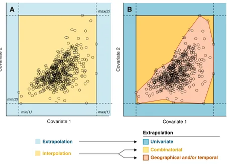
Extrapolation detection methods are typically extrinsic (i.e. independent of the model itself) (Grenier et al. 2013) , with the most common being to interpret predictions relative to the numerical range of each covariate entering the model. Predictions at covariate values outside the range of observed data are labelled as ‘extrapolations’, and those within the range are denoted ‘interpolations’ (Qiao et al. 2019) ( Fig. 8 A ). Many studies have shown that predictive accuracy is impaired when a model is extrapolated to new sites or time periods (Torres et al. 2015; Roach et al. 2017; Sequeira et al. 2018b) , making this dichotomy appealing for identifying subsets of predictions that can reasonably be expected to be less reliable, all things being equal (Randin et al. 2006; Heikkinen et al. 2012) .

Covariate values, however, are rarely distributed homogeneously in covariate space ( Fig. 8 A ). Even predictions classed as ‘interpolations’ (light yellow area in Fig. 8 A ) may include novel combinations of values not encountered in the original sample (Mesgaran et al. 2014) . A more nuanced typology of extrapolation is required that recognises the reference points as occupying a discrete volume (i.e. envelope) within the hyperspace of modelled covariates. The simplest delineation of this envelope is a hyperpolyhedron (i.e. convex hull) or an ellipsoid that encompasses the most extreme observations of each covariate (King & Zeng 2007; García-López & Allué 2013) .

It follows that three types of extrapolation can be identified ( Fig. 8 B ):

● Univariate extrapolation, which identifies out-of-range values for any given covariate. Also known as mathematical, strict, novel or Type 1 extrapolation (dark blue in Fig. 8 B ).

● Combinatorial extrapolation, which detects novel combinations of values encountered within the univariate range of reference covariates. Also known as multivariate, novel-combination, or Type 2 extrapolation (dark yellow in Fig. 8 B ).

Figure 8 : Typology of environmental extrapolation, with black circles denoting reference samples. (A)

Simple binary classification defined in the bivariate space of two hypothetical environmental covariates. Interpolation here occurs when points fall within the rectangle defined by the minimum and maximum values of individual covariates (light yellow). Extrapolation takes place outside that rectangle (light blue).

(B) Refined classification that also considers novel combinations of covariates (dark yellow), as per Mesgaran et al. (2014) . By contrast, out-of-range predictions are now termed ‘univariate’ extrapolations. Any points within the envelope (red outline) of the sampled data correspond to conditions analogous to those found in the reference system, and are termed ‘Geographical/temporal extrapolation’ if found in a different region or time slice.

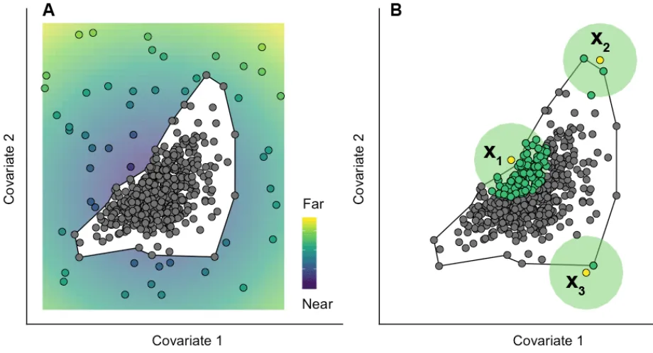
space; or conversely, for two target points reflecting an equal degree of extrapolation stricto sensu to contain very different amounts of reference data in their vicinity. An example of this is shown in Fig. 9 B , where three target points , , and , are located at equal distances to the envelope of the reference data.

Figure 9 : Conceptual representation of two key extrapolation metrics. (A) Distance from the envelope (black polygon) of the reference data (grey circles). A target point located far outside the sampled environmental space (e.g. falling in the yellower areas) is more dissimilar and therefore ‘more of an extrapolation’ than one closer to it (e.g. falling in the bluer areas). (B) Neighbourhood (or ‘percentage of data nearby’). Owing to the complex shape of the reference data cloud in multivariate space, the amount of sample information available to ‘inform’ predictions made at target points can vary considerably. For instance, contrast the proportion of reference data points (in green) contained within comparable radii of prediction points and .

ExDet harnesses the properties of a scale-invariant measure of multivariate outliers, the   Mahalanobis distance, to characterise the degree of novelty/similarity between reference and target domains. Doing so gives ExDet a number of advantages (Farber & Kadmon 2003) :

● It is relevant to both orthogonal and correlated covariates, and can accommodate the latter even if they exhibit heterogeneous variances. Mathematically, the Mahalanobis distance reduces to a standardised Euclidean distance when the covariance between variables approaches zero (i.e. variables are orthogonal to each other) (Mahony et al. 2017) .

● It accounts for different dispersions between covariates through standardisation.

● It is robust to departures from multivariate normality.

● It allows a natural definition of the most influential covariates (MIC), i.e. those that make the largest contribution to extrapolation in the target system.

● It has a clear theoretical basis that aligns with the principle of central tendency as expressed in niche theory (Whittaker 1975) , which suggests that species’ survival is maximised in optimal conditions and reduces to zero outside environmental tolerance limits.

Furthermore, ExDet simultaneously accounts for both univariate and combinatorial extrapolation, yielding a more comprehensive picture of extrapolation that is lacking from other metrics or otherwise difficult to obtain in a manner functional for model end-users (Mesgaran et al. 2014) . Addressing combinatorial extrapolation is especially important as model predictions may only be reliable where collinearity patterns among covariates remain stable (Rödder & Engler 2012) . Note that, by design, ExDet only detects combinatorial extrapolation within the rectilinear envelope of input covariates ( Fig. 8 B ), however extensions to the framework have recently been proposed to broaden its applicability (Muthoni et al. 2017) . Note also that Mahalanobis distances vary as a function of the number of selected covariates. The effect of covariate dimensionality on ExDet outputs is therefore a critical consideration for their correct interpretation (Mahony et al. 2017) . Small covariate sets should carry lower risk of false positives (akin to Type I inference errors), but at the cost of potentially higher rates of false negatives (akin to Type II errors) (Mahony et al. 2017) . In the absence of abundance data in the target system, it is hard to find an objective basis for choosing a specific covariate set over another, other than purely through ecological reasoning. That said, it can be shown the distribution of Mahalanobis distances for multivariate normal data is approximated by a distribution with degrees of freedom, where equals the number of covariates/dimensions (Clark et al. 1993; Farber & Kadmon 2003) . It follows that Mahalanobis distances can be

expressed probabilistically as percentiles of the distribution (Mahony et al. 2017) , allowing a more transparent and meaningful interpretation of the significance of extrapolation.

overlooked dimension of extrapolation. Typically, the geometric variability present in the reference sample acts as a rule of thumb threshold, such that prediction points are considered ‘nearby’ if they sit within one geometric mean Gower’s distance of the data (the mean value being calculated between all pairs of reference points; King & Zeng 2007) . %N has the benefit of being applicable to both quantitative and qualitative variables, and has been used with success in previous studies of cetacean populations (Virgili et al. 2017; Mannocci et al. 2018; García-Barón et al. 2019) .

3. Software

This report is accompanied by a vignette covering practical examples of extrapolation assessments for both sperm whale ( Physeter macrocephalus ) and beaked whale ( Ziphiidae spp ) DSMs in popular software R. The data used in the case studies come from shipboard and aerial line transect surveys undertaken across the North Atlantic and Gulf of Mexico, and are fully described in Roberts et al. (2016) and Mannocci et al. (2017b) .

At present, the R code is provided in the ExDet-functions.R file, and comprises the following key functions:

● ExDet : An adaptation of the ecospat.climan function from the ecospat package (formerly ecospat.exdet in previous releases of the package). It is used to assess the degree of environmental similarity between a reference and a target system, as described in Mesgaran et al. (2014) , with the added functionality of identifying the most influential covariate(s) - MIC - i.e. contributing most to departures from reference conditions.

● whatif.opt : An adaptation of the whatif function from the WhatIf package (Stoll et al. 2005) , modified to run on large datasets via matrix partitioning.

● compute_extrapolation : This function calls ExDet and returns results in both data.frame and raster formats.

● summarise_extrapolation : Function to summarise extrapolation results in tabular form. It is called internally by compute_extrapolation by default.

● compare_covariates : This is a wrapper around compute_extrapolation that can used to assess extrapolation for different combinations of covariates, as a means of informing covariate selection during model development.

● compute_nearby : This is a wrapper around whatif and whatif.opt that quantifies the proportion of reference points located in the vicinity of each target point in multivariate space, as an additional metric of extrapolation. See King and Zeng (2007) for details.

● Map_extrapolation : This function supports the visual assessment of extrapolation by generating interactive html maps of the outputs from compute_extrapolation.

● Extrapolation_analysis : This function allows a full assessment of extrapolation (i.e. calculations, summary, and visualisation) to be conducted in one single run, by combining calls to compute_extrapolation, summarise_extrapolation, and map_extrapolation.

Note that work is underway to compile this code into an R package to be made available on CRAN in 2019. Both the R code and the vignette are available from

4. Outlook and recommendations

Pressing needs to tackle the challenges posed by climate warming, habitat loss, and species extinctions have spurred strong demands for ecological models that can help elucidate wildlife abundance and distribution patterns across a variety of scales, and to foresee the responses of biodiversity to multiple drivers of change (Coreau et al. 2009; Mouquet et al. 2015; Maris et al. 2018) . However, despite sustained efforts to survey the Earth's’ biomes over the last decades (Costello et al. 2010) , detailed occurrence or density maps are still unavailable for most taxa (Green et al. 2005) . In the wake of a worldwide economic crisis, cuts in conservation spending are also forcing agencies responsible for biological data collection to operate on shoestring budgets, limiting the scope of further monitoring and field sampling to smaller areas, shorter and more irregular time spans, and cheaper assessment methods (Borja & Elliott 2013) . As anthropogenic impacts on ecosystems continue to accelerate, there is hence increasing appetite for translating sporadic ecological understanding accumulated at local or regional levels into broad-scale insights that can facilitate strategies to manage and adapt to the effects of global change (Heffernan et al. 2014) . This makes extrapolation a pivotal – if not imperative – component of research agendas in applied ecology (Colwell & Coddington 1994; Clark et al. 2001) , particularly within the marine arena (e.g. Redfern et al. 2017; Péron et al. 2018; Sequeira et al. 2018a) .

We adopt a more optimistic viewpoint; one that acknowledges predictions as a useful way of testing and demonstrating ecological understanding (Houlahan et al. 2017) , and that recognises accurate forecasting as a hallmark of successful science (Evans et al. 2012) . We argue that, when exercised with due diligence, extrapolation can be a powerful driver of scientific conjecture and discovery (Coreau et al. 2009) , such that methods supporting the projection of models into novel conditions are paramount to catalysing future advances in fields like conservation planning, agriculture, engineering or epidemiology (Acevedo et al. 2014) . One of the greatest obstacles to extrapolating well-fitted DSMs to novel conditions, of course, is the lack of target data with which to validate predictions in many information-poor ecosystems (e.g. Redfern et al. 2017) . Counter-intuitively, extrapolation is both a consequence of, and a solution to, data deficiency in this context. By projecting models, we can generate null hypotheses against which new data can subsequently be checked (as and when they become available), allowing extrapolation to serve as an instrument of learning that fosters long-term improvements in predictive ability (Petchey et al. 2015; Pennekamp et al. 2017) . Extrapolation can also be strategically applied to the formulation of survey designs, and one could easily think of augmenting a sampling scheme with a number of sites expected to exhibit high prediction variance (Conn et al. 2015a) , or simply guiding survey efforts to those areas with higher probabilities of species occurrence or abundance (Bourke et al. 2012; Mannocci et al. 2018) .