Chaos synchronization between two identical restricted three body problem via active control and adaptive control method

_______________

*_{Corresponding author}

E-mail address: [email protected] Received January 15, 2019

Available online at http://scik.org

J. Math. Comput. Sci. 9 (2019), No. 3, 288-302 https://doi.org/10.28919/jmcs/3996

ISSN: 1927-5307

CHAOS SYNCHRONIZATION BETWEEN TWO IDENTICAL RESTRICTED THREE BODY PROBLEM VIA ACTIVE CONTROL AND ADAPTIVE

CONTROL METHOD

MOHD ARIF*

Zakir Husain Delhi College (Delhi University), Jawaharlal Nehru Marg N. Delhi-2, India

Copyright © 2019 the author(s). This is an open access article distributed under the Creative Commons Attribution License,which permits unrestricted use, distribution, and reproduction in any medium, provided the original work is properly cited.

Abstract: This article presents the chaos synchronization problem of the restricted three body problem (RTBP) when the massive primary is supposed to be oblate spheroid and the smaller one is a uniform circular ring. The feedback controller for the stability of the closed-loop system are designed using the active control and adaptive control strategy. It is shown that the two methods have excellent performance, with the active control marginally outperforming the adaptive control in terms of transient analysis. Simulation results satisfy the theoretical findings. For validation of results by numerical simulations, the Mathematica 10 is used when the primaries are Saturn and Jupiter.

Keywords:chaos; synchronization; active control; adaptive control; restricted three body problem. 2010 AMS Subject Classification: 70P05, 37N35.

1.

I

CHAOS SYNCHRONIZATION

master and slave system and they demonstrated that chaotic synchronization could be achieved by driving or replacing one of the variables of a chaotic system with a variable of another similar chaotic device. Many methods for chaos synchronization of various chaotic systems have been developed, such as non linear feedback control [2], OGY approach [3], sliding mode control [4], anti synchronization method [5], adaptive synchronization [6], active control [7] and so on. The active control methods for synchronizing the chaotic systems has been applied to many practical systems such as spatiotemporal dynamical systems (Codreanu [8]), the Rikitake two-disc dynamo-a geographical systems (Vincent 9]), Complex dynamos (Mahmoud [10]) and Hyper-chaotic and time delay systems (Israr Ahmad et al. [11]) etc. Shihua Chen and Jinhu [12] proposed a new adaptive control method for adaptive synchronization of two uncertain chaotic systems, using a speci_c uncertain uni_ed chaotic model.

Many mathematicians have investigated the circular restricted three body problem such as the Euler [13], Hill [14], Poincare [15], Lagrange [16], Deprit [17], Hadjidemetriou [18], Bhatnagar [19,20], Sharma et al. [21,22], Sahoo and Ishwar [23] and many others. These studies focus on the analytical, qualitative and numerical studies of the problem. A detailed analysis of this problem is illustrated in the work of American mathematician Szebehely [24]. Khan and Shahzad [25] investigated the synchronization behavior of the two identical circular restricted three body problem inuenced by radiation evolving from di_erent initial conditions via the active control Arif [26] studied the complete synchronization, anti-synchronization and hybrid synchronization in the planar restricted three p0roblem by taking into consideration the small primary is ellipsoid and bigger primary an oblate spheroid via active control technique.

master system in the course of time. The paper is organized as follows. In section 2 we derive the equations of motion of the system. Section 3 deals with the complete synchronization of the problem via active control and section 4 via adaptive control. Finally, we conclude the paper in section 5.

2.

Equation of motion

The equation of motion for the restricted three body problem when the massive primary is supposed to be oblate spheroid and the smaller one is a uniform circular ring in a dimensionless rotating, co-ordinate system are as follows,

𝑥̈ − 2 𝜔 𝑦̇ = 𝑈_𝑥 (1)

𝑦̈ + 2 𝜔 𝑥̇ = 𝑈_𝑦 (2) Where

𝑈𝑥 =𝜕𝑈_𝜕𝑥 and 𝑈𝑦 = 𝜕𝑈_𝜕𝑦 𝑈 = 𝜔₂2 (𝑥2 _{+ 𝑦}2_{) + {}1−µ

r1 +

𝐼 2 𝑟₁3} +

2 µ

π (𝑎2_−𝑏2₎ [(𝑏 + r2) 𝐸(𝜃, 𝑘𝑏) + (𝑏 − r2) 𝐾(𝜃, 𝑘𝑏) −

(𝑎 + r2) 𝐸(𝜃, 𝑘𝑎) − (𝑎 − r2) 𝐾(𝜃, 𝑘𝑎)] (3) 𝜔 = mean motion of the primaries, µ = mass ratio, 𝑎, 𝑏 = outer and inner radii of the ring

respectively. 𝐼 = µ(R2_e− R_p2)/5, 𝑅_𝑒 , 𝑅_𝑝 equatorial and polar radius of oblate spheroid respectively.

K(𝜃, 𝑘𝑎,𝑏) = ∫ dθ

√1−𝑘_𝑎,𝑏2 𝑠𝑖𝑛2_𝜃 π

2

0 Elliptic integral of first kind,

E(𝜃, 𝑘_𝑎,𝑏) = ∫ √1 − 𝑘π2 _𝑎,𝑏2 _𝑠𝑖𝑛2_{𝜃 dθ}

0 Elliptic integral of second kind, 𝑘𝑎 =

√4𝑎r2

(𝑎+r2) , 𝑘𝑏 =

√4br2

(b+r2) .

𝑟₁2_{= (𝑥 − µ)}2_{+ 𝑦}2_{, 𝑟}

22 = (𝑥 + 1 − µ)2+ 𝑦2.

The only integral of motion available for the system of equations 1and 2 is the Jacobi constant

𝑥̇2 _{+ 𝑦̇}2 _{= 2U − C (4)}

CHAOS SYNCHRONIZATION

forbidden region and allowed regions of motion bounded by the Hill’s surfaces. Let S be that energy surface,

i.e.,

𝑆(𝜇, 𝐶) = {(𝑥, 𝑦, 𝑥̇, 𝑦̇ )| 𝐶(𝑥, 𝑦, 𝑥̇, 𝑦̇ ) = 𝑐𝑜𝑛𝑠𝑡𝑎𝑛𝑡} (5)

The projection of this surface onto position space is called a Hill's region

𝑆(𝜇, 𝐶) = {(𝑥, 𝑦)| U(𝑥, 𝑦 ) ≥𝐶₂}. (6)

The boundary of 𝑆(𝜇, 𝐶) is the zero velocity curve. The negligible mass can move only within this region in the (𝑥, 𝑦)-plane. There are basic two configurations for the Hill's region for a given value of 𝜇.

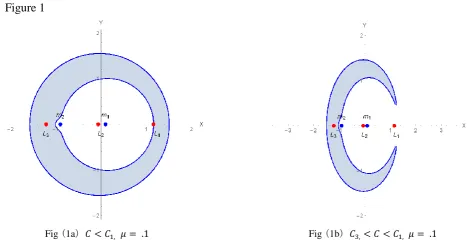
Figure 1

Fig (1a) 𝐶 < 𝐶1, 𝜇 = .1 Fig (1b) 𝐶3,< 𝐶 < 𝐶1, 𝜇 = .1

The values of C which separate these two cases will be denoted 𝐶_𝑖 𝑖 = 1,3 which are the values corresponding to the equilibrium points 𝐿₁ and 𝐿₃. These values can be easily calculated for small 𝜇 and their graphs are shown in Figure 1. For case 2, the Jacobi constant lies between

𝐶1 and 𝐶3 which are the Jacobi constants of the libration points 𝐿1 and 𝐿3 respectively. In

3.

Synchronization via Active Control

Let

𝑥 = 𝑥₁, 𝑥̇ = 𝑥₂, 𝑦 = 𝑥₃, 𝑦̇ = 𝑥₄

Then the equation (1) and (2) can be written as:

𝑥̇₁ = 𝑥₂ (7)

𝑥̇₂ = 2𝜔𝑥₄ + 𝜔2_𝑥

1+ 𝐴1 (8) 𝑥̇₃ = 𝑥₄ (9)

𝑥̇4 = −2𝜔𝑥2+ 𝜔2𝑥3 + 𝐴2 (10)

Where

𝐴1 =

−(1 − µ )(𝑥₁− µ)

r₁3 −

3 I (𝑥₁− µ) 2r₁5

− 2 µ (𝑥1+ 1 − µ) 𝜋(𝑎2_{− 𝑏}2_{) 𝑟}

2 [(E(𝜃, 𝑘𝑏) − K(𝜃, 𝑘𝑏)) (1 +

4𝑏(𝑏 − 𝑟2) 𝑘_𝑏(𝑏 + r₂2₎)

+4𝑏(𝑏 − 𝑟2) 2

(𝑏 + 𝑟2)3 (

(E(𝜃, 𝑘𝑏) − (1 − 𝑘𝑏2)K(𝜃, 𝑘𝑏))

𝑘_𝑏(1 − 𝑘_𝑏2) )

+ (E(𝜃, 𝑘𝑎) − K(𝜃, 𝑘𝑎)) (1 +

4𝑎(𝑎 − 𝑟₂) 𝑘_𝑎(𝑎 + r₂2₎)

+4𝑎(𝑎 − 𝑟2)2 (𝑎 + 𝑟₂)3 (

(E(𝜃, 𝑘_𝑎) − (1 − 𝑘_𝑏2)K(𝜃, 𝑘_𝑎))

𝑘_𝑎(1 − 𝑘_𝑎2) )]

𝐴₂ =−(1−µ )𝑥3

r₁3 −

3I 𝑥3

2r₁5 −

2 (µ) 𝑥3

𝜋(𝑎2_−𝑏2_{) 𝑟2}[(E(𝜃, 𝑘𝑏) − K(𝜃, 𝑘𝑏)) (1 +

4𝑏(𝑏−𝑟2)

𝑘𝑏(𝑏+r22)) +

4𝑏(𝑏−𝑟2)2

(𝑏+𝑟2)3 (

(E(𝜃,𝑘𝑏)−(1−𝑘𝑏2)K(𝜃,𝑘𝑏))

𝑘𝑏(1−𝑘𝑏2) ) + (E(𝜃, 𝑘𝑎) − K(𝜃, 𝑘𝑎)) (1 +

4𝑎(𝑎−𝑟2)

𝑘𝑎(𝑎+r22)) +

4𝑎(𝑎−𝑟2)2

(𝑎+𝑟2)3 (

(E(𝜃,𝑘𝑎)−(1−𝑘𝑏2)K(𝜃,𝑘𝑎))

𝑘𝑎(1−𝑘𝑎2) )]

𝑟₁2= (𝑥₁− µ)2+ 𝑥₃2, 𝑟₂2 = (𝑥₁+ 1 − µ)2+ 𝑥₃2.

CHAOS SYNCHRONIZATION

Fig(2)

Corresponding to master system ((7), … (10)), the identical slave system is defined as:

𝑦̇₁ = 𝑦₂+ 𝑢₁(𝑡) (11)

𝑦̇₂ = 2𝜔𝑦₄+ 𝜔2𝑦₁+ 𝐵₁+ 𝑢₂(𝑡) (12)

𝑦̇₃ = 𝑦₄ +𝑢₃(𝑡) (13)

𝑦̇4 = −2𝜔𝑦2+ 𝜔2𝑦3+ 𝐵2+ 𝑢4(𝑡) (14)

Where

𝐵1 =

−(1 − µ )(𝑦₁− µ)

r₁₁3 −

3 I (𝑦₁− µ) 2r₁₁5

− 2 (µ) (𝑦1+ 1 − µ) 𝜋(𝑎2_{− 𝑏}2_{) 𝑟}

21 [(E(𝜃, 𝑘𝑏) − K(𝜃, 𝑘𝑏)) (1 +

4𝑏(𝑏 − 𝑟21) 𝑘_𝑏(𝑏 + r₂₁2 ₎)

+4𝑏(𝑏 − 𝑟21) 2

(𝑏 + 𝑟21)3 (

(E(𝜃, 𝑘𝑏) − (1 − 𝑘𝑏2)K(𝜃, 𝑘𝑏))

𝑘_𝑏(1 − 𝑘_𝑏2) )

+ (E(𝜃, 𝑘𝑎) − K(𝜃, 𝑘𝑎)) (1 +

4𝑎(𝑎 − 𝑟₂₁) 𝑘𝑎(𝑎 + r212 ) )

+4𝑎(𝑎 − 𝑟21)2 (𝑎 + 𝑟₂₁)3 (

(E(𝜃, 𝑘_𝑎) − (1 − 𝑘_𝑏2)K(𝜃, 𝑘_𝑎))

𝑘_𝑎(1 − 𝑘_𝑎2) )]

4000 2000 2000 4000 x

𝐵2 = −(1−µ )𝑦_r 3

11 3 −

3 I 𝑦3

2r115 −

2 (µ) 𝑦3

𝜋(𝑎2_−𝑏2_{) 𝑟21}[(E(𝜃, 𝑘𝑏) − K(𝜃, 𝑘𝑏)) (1 +

4𝑏(𝑏−𝑟21)

𝑘𝑏(𝑏+r212 )) +

4𝑏(𝑏−𝑟21)2

(𝑏+𝑟21)3 (

(E(𝜃,𝑘𝑏)−(1−𝑘𝑏2)K(𝜃,𝑘𝑏))

𝑘𝑏(1−𝑘𝑏2) ) + (E(𝜃, 𝑘𝑎) − K(𝜃, 𝑘𝑎)) (1 +

4𝑎(𝑎−𝑟21)

𝑘𝑎(𝑎+r212 )) +

4𝑎(𝑎−𝑟21)2

(𝑎+𝑟21)3 (

(E(𝜃,𝑘𝑎)−(1−𝑘𝑏2)K(𝜃,𝑘𝑎))

𝑘𝑎(1−𝑘𝑎2) )]

𝑟₁₁2= (𝑦₁− µ)2+ 𝑦₃2, 𝑟₂₁2 = (𝑦₁+ 1 − µ)2+ 𝑦₃2.

where 𝑢_𝑖(𝑡); 𝑖 =1 ,2,3,4 are control functions to be determined.

Let 𝑒_𝑖 = 𝑦_𝑖 − 𝑥_𝑖 ; i = 1, 2, 3, 4 be the synchronization errors. From ((7)….(10)) and ((11)….(14)), we obtain the error dynamics as follows:

𝑒1̇ = 𝑒2+ 𝑢1(𝑡) (15)

𝑒₂̇ = 2𝜔𝑒₄ + 𝜔2_𝑒

1+ 𝐵1− 𝐴1+ 𝑢2(𝑡) (16) 𝑒₃̇ = 𝑒₄ + 𝑢₃(𝑡) (17)

𝑒₄̇ = −2𝜔𝑒₂+ 𝜔2_𝑒

3+ 𝐵2− 𝐴2 + 𝑢4(𝑡) (18)

Let us redefine the control functions so that the terms in (15) to (18) which cannot be expressed as linear terms in 𝑒_𝑖's are eliminated :

𝑢1(𝑡) = 𝑣1(𝑡)

𝑢₂(𝑡) = −𝐵₁+ 𝐴₁+ 𝑣₂(𝑡) 𝑢3(𝑡) = 𝑣3(𝑡)

𝑢4(𝑡) = −𝐵2+ 𝐴2+ 𝑣4(𝑡)

The new error system can be expressed as:

𝑒₁̇ = 𝑒₂+ 𝑣₁(𝑡)

𝑒₂̇ = 2𝜔𝑒₄ + 𝜔2_𝑒

1+ 𝑣2(𝑡) 𝑒₃̇ = 𝑒₄ + 𝑣₃(𝑡)

𝑒4̇ = −2𝜔𝑒2+ 𝜔2𝑒3+ 𝑣4(𝑡)

The above error system to be controlled is a linear system with a control input 𝑣_𝑖(𝑡) ( 𝑖 =

1, … 4) as function of the error states 𝑒_𝑖 ( 𝑖 = 1, … 4). As long as these feedbacks stabilize the system 𝑒_𝑖 ( 𝑖 = 1, … 4) converge to zero as time 𝑡 tends to infinity. This implies that master

CHAOS SYNCHRONIZATION

[ 𝑣1(𝑡) 𝑣₂(𝑡) 𝑣3(𝑡) 𝑣₄(𝑡)

] = 𝐴 [ 𝑒1 𝑒2 𝑒₃ 𝑒₄ ]

Here 𝐴 is a 4 × 4 coefficient matrix to be determined. As per Lyapunov stability theory and Routh-Hurwitz criterion, in order to make the closed loop system (20) stable, proper choice of elements of 𝐴 has to be made so that the system (20) must have all eigen values with negative real parts. Choosing

𝐴 = [

−1 −1 0 0

−𝜔2 _{−1 0 −2𝜔}

0 0 −1 −1

0 2𝜔 −𝜔2 ₋₁

]

and, defining a matrix 𝐵 as

[ 𝑒1̇ 𝑒₂̇ 𝑒3̇ 𝑒4̇

] = 𝐵 [ 𝑒1 𝑒2 𝑒3 𝑒4 ]

Where 𝐵 is

𝐵 = [

−1 0 0 0

0 −1 0 0

0 0 −1 0

0 0 0 −1

]

Clearly, 𝐵 has eigen values with negative real parts. This implies lim

𝑡→∞|𝑒𝑖| = 0; 𝑖 = 1, 2, 3, 4

and hence, complete synchronization is achieved between the master and slave systems.

4. Synchronization via Adaptive Control

In this section we design an adaptive controller for the slave system (11)...(14). Lyapunov stability theory state that when controller satisfies the assumption with V (e) = 1₂ 𝑒𝑡𝑒 a positive definite function and the first derivative of this function 𝑉̇< 0, the chaos synchronization of two identical systems (master and slave) for different initial conditions is achieved. Construct a Lyapunov function as:

(20)

(21)

(22)

𝑉̇ =1₂(𝑒₁2_{+ 𝑒}

22+ 𝑒32+ 𝑒42).

Then its derivative along the error system (15) to (18) is

𝑉̇ = 𝑒1(𝑒2+ 𝑢1) + 𝑒2{2𝜔𝑒4+ 𝜔2𝑒1+ 𝐵1− 𝐴1+ 𝑢2} + 𝑒3(𝑒4+ 𝑢3) +𝑒₄{−2𝜔𝑒2+ 𝜔2𝑒3+ 𝐵2− 𝐴2+ 𝑢4} .

Hence, if we choose the controller 𝑢 as follows,

𝑢₁ = −𝑒₁− 𝑒₂

𝑢2 = −𝜔2𝑒1− 𝐵1+ 𝐴1− 𝑒2

𝑢₃ = −𝑒₃− 𝑒₄

𝑢4 = −𝜔2𝑒3− 𝐵2+ 𝐴2− 𝑒4

Then

𝑉̇ = −𝑒12− 𝑒22− 𝑒32− 𝑒42 < 0.

Hence the error state

lim

𝑡→∞‖𝑒(𝑡)‖ = 0.

which gives asymptotic stability of the system. This means that the controlled chaotic systems (master and slave) are synchronized for deferent initial conditions.

NUMERICAL SIMULATION

Let us consider an example of Jupiter-Saturn system in the restricted three body problem in which the primary 𝑚₂is taken as the Saturn and primary 𝑚₁ as the Jupiter and small body as a space- craft. From the astrophysical data we have

Mass of the Saturn 𝑚₂ = 5:683 × 1026kg Mass of the Jupiter 𝑚1 = 1:89712 × 1027kg

The distance between the Jupiter and Saturn = 646,270,000 Km.

In dimensionless system we have 𝑚1+𝑚2 = 1 unit and the distance between the Jupiter-Saturn

is 1 unit.

CHAOS SYNCHRONIZATION

controlled system Via active control are shown in figures 4,7,10 and 13 and via Adaptive control are shown in figures 5,8,11,14 respectively. These figures shows that the state [𝑥₁(𝑡), 𝑥₂(𝑡),

𝑥₃(𝑡), 𝑥₄(𝑡)] of master system [7 to 10] asymptotically synchronize with the state [𝑦₁(𝑡), 𝑦₂(𝑡),

𝑦₃(𝑡), 𝑦₄(𝑡)]of slave system [11 to 14]. Fig. (15) shows the synchronization error (e) for the two system. We find that at t = 6s, the synchronization was already attained for adaptive control while synchronization was attained at a later time (t = 10s) for active control, the time delay being 4 s. Though it is clear that the adaptive control performs better and is much easier to design.

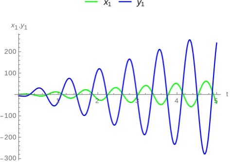
Fig (3): Time series of the Uncontrolled states 𝑥1, 𝑦1.

Fig (4): Time series of the controlled states 𝑥1, 𝑦1via Active control Fig (5): Time series of the controlled states 𝑥1, 𝑦1via Adaptive control

x1 y1

1 2 3 4 5 t

300 200 100 100 200

x₁,y₁

x1 y1 x1 y1

0.5 1.0 1.5 2.0 2.5 3.0 t

40 30 20 10 10 20 30

x₁,y₁

0.5 1.0 1.5 2.0 2.5 3.0 t

40 30 20 10 10 20 30

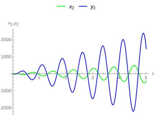
Fig (6) :Time series of the Uncontrolled states 𝑥2, 𝑦2.

Fig (7) :Time series of the controlled states 𝑥2, 𝑦2via Active control Fig (8) :Time series of the controlled states 𝑥2, 𝑦2via Adaptive control

x2 y2

1 2 3 4 5 t

2000 1000 1000 2000

x₂,y₂

x2 y2 x2 y2

0.5 1.0 1.5 2.0 2.5 3.0 t

300 200 100 100 200 300

x₂,y₂

0.5 1.0 1.5 2.0 t

200 100 100

CHAOS SYNCHRONIZATION

Fig (9) :Time series of the Uncontrolled states 𝑥3, 𝑦3.

Fig (10) :Time series of the controlled states 𝑥2, 𝑦2via Active control Fig (11) :Time series of the controlled states 𝑥2, 𝑦2via Adaptive control

Fig (12) :Time series of the Uncontrolled states 𝑥3, 𝑦3.

x3 y3

1 2 3 4 5 t

200 100 100 200 300

x₃,y₃

x3 y3 x3 y3

0.5 1.0 1.5 2.0

t

20 10 10 20

x₃,y₃

0.5 1.0 1.5 2.0

t

20 10 10 20

x3 ,y3

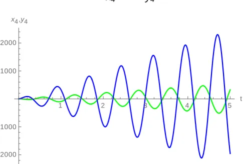
x4 y4

1 2 3 4 5 t

2000 1000 1000 2000

Fig (13) :Time series of the controlled states 𝑥2, 𝑦2via Active control Fig (14) :Time series of the controlled states 𝑥2, 𝑦2via Adaptive control

Fig (15a) :Error system via Active control Fig ( 15 b) :Error system via Adaptive control

5. Conclusions

The equation of motion of the restricted three-body problem when the massive primary is supposed to be oblate spheroid and the smaller one is an uniform circular ring formulated. We have investigated the complete synchronization behavior of the problem via adaptive and active control method. Here two systems (master and slave) are compete synchronized when start with deferent initial conditions. Hence the slave chaotic system completely traces the dynamics of the master system in the course of time. For validation of results by numerical simulations we used

x4 y4 x4 y4

0.5 1.0 1.5 2.0

t

200 100 100

x4,y4

0.5 1.0 1.5 2.0 t

200 100 100 200

x₄,y₄

e11Adaptive control e21 Adaptive control e31Adaptive control e41 Adaptive control

2 4 6 8 10 12 14 t

0.1 0.2 0.3 0.4 0.5

e_{1 ,}e_{2 ,}e_{3 ,}e₄

2 4 6 8 10 12 14 t

0.1 0.2 0.3 0.4 0.5 0.6 0.7 e₁,e₂,e₃,e₄

CHAOS SYNCHRONIZATION

the Mathematica 10 when the primaries are Jupiter and Saturn. Conflict of Interests

The authors declare that there is no conflict of interests.

REFERENCES

[1] Pecora L. M.,Carroll T.L., Synchronization in chaotic systems, Rev. Lett. 64 (1990), 821- 824.

[2] Lu L., Zhang C., Guo Z. A. Synchronization between two different chaotic systems with non linear feedback control, Chinese Phys. 16-6 (2007), 1603-1607.

[3] Ott., Grebogi C., Yorke J. A. Controlling Chaos, Phys. Rev. Lett., 64 (1990), 1196-1199.

[4] Haeri M., Emadzadeh A. Synchronizing different chaotic systems using active sliding mode control, Chaos Solitons Fractals, 1 (2003). 119-129.

[5] Park J. H., Chaos synchronization between two different chaotic dynamical systems. Chaos Solitons Fractals, 27-2 (2006), 549-554.

[6] Wang Y., Guan Z. H.,Wang H. O., Feedback and adaptive control for the synchronization of Chen system via a single variable, Phys. Lett. , 312-1 (2003), 30-40.

[7] Bai E.W., Lonngren K.E., Synchronization of two Lorenz systems using active control, Chaos Solitons Fractals, 8 (1997), 51-58.

[8] Codreanu, S., Synchronization of spatiotemporal nonlinear dynamical systems by an active control. Chaos Solitons Fractals, 15 (2003), 507-510.

[9] Vincent, U. E., Synchronization of Rikitake chaotic attractor via active control. Phys. Lett. A, 343 (2005), 133-138.

[10]Mahmoud, G. M., Aly, S. A. and Farghaly, A. On chaos synchronization of a complex two coupled dynamos system. Chaos Solitons Fractals, 33 (2007), 178-187.

[12] Shihua Chen, Jinhu Leu., Synchronization of an uncertain unified chaotic system via adaptive control. Chaos Solitons Fractals 14 (2002), 643–647.

[13]Euler, L., Un corps etant attire en raison reciproque quarree des distances vers deux points fixes donnes. Mem. Berlin (1760), 228.

[14]Hill, G. W., Reasearches in the lunar theory. Am. J. Math. 1 (1878). [15]Poincare, H., Sciences et Methode. (1908).

[16]Lagrange, J. Ocuvres 14, vols Gauthier-Villars, Paris. (1772).

[17]Deprit A. and Price J. F., The computation of characteristic exponents in the planar restricted three body problem. Astro. J.,70 (1964), 836-849.

[18]Hadjidemetriou, J. D., Asteroid motion near the 3:1. Celest Mech. Dyn. Astron., 56 (1- 2) (1993), 201-219. [19]Bhatnagar, K. B., Periodic orbits of collision in the restricted problem of three bodies in a three-dimensional

co-ordinate system. Ind. J. Pure Appl. Math., 3 (1) (1969), 101-117.

[20]Bhatnagar, K. B. and Chawla, J. M., A study of the Lagrangian points in the photogravitational restricted three body problem. Ind. J. Pure Appl. Math., 10(11) (1979), 1443-1451.

[21]Sharma, R. K. and Subbarao, collinear equilibria and their characteristic exponents in the restricted three body problem when the primaries are oblate spheroids. Celestial Mechanics, 12 (1975), 189-201.

[22]Sharma, R. K., Taqvi, Z. A. and Bhatnagar, K.B., Existence and stability of the libration point of the restricted three body problem when the bigger primary is a triaxial body and a source of radiation. Indian J. Pure Appl. Math. 32(2) (2001), 255-266.

[23]Sahoo, S. k. and Ishwar, B., Stability of the collinear equilibrium points in generalized the photogravitational elliptical restricted three body problem. Bull Astr. Soc. India, 28, (2000), 579-586.

[24]Szebehely, V., Theory of Orbits., Academic press, New York. (1967).

[25]Khan, A., Shahzad, M., Chaos Synchronization in a Circular Restricted Three Body Problem Under the Effect of Radiation. Chaos Complex Syst. (2012), 59-68.