Porting marine ecosystem model spin-up using transport matrices to GPUs

(1)

Geosci. Model Dev., 6, 17–28, 2013 www.geosci-model-dev.net/6/17/2013/ doi:10.5194/gmd-6-17-2013

Geoscientific

Model Development

Porting marine ecosystem model spin-up using transport matrices

to GPUs

E. Siewertsen1, J. Piwonski2, and T. Slawig2

1_{Institute for Computer Science, Christian-Albrechts Universit¨at zu Kiel, 24098 Kiel, Germany}

2_{Institute for Computer Science and Kiel Marine Science – Centre for Interdisciplinary Marine Science,}

Cluster The Future Ocean, Christian-Albrechts Universit¨at zu Kiel, 24098 Kiel, Germany

Correspondence to: T. Slawig ([email protected])

Received: 19 July 2012 – Published in Geosci. Model Dev. Discuss.: 31 July 2012 Revised: 7 November 2012 – Accepted: 5 December 2012 – Published: 8 January 2013

Abstract. We have ported an implementation of the spin-up for marine ecosystem models based on transport matrices to graphics processing units (GPUs). The original implementa-tion was designed for distributed-memory architectures and uses the Portable, Extensible Toolkit for Scientific Compu-tation (PETSc) library that is based on the Message Passing Interface (MPI) standard. The spin-up computes a steady sea-sonal cycle of ecosystem tracers with climatological ocean circulation data as forcing. Since the transport is linear with respect to the tracers, the resulting operator is represented by matrices. Each iteration of the spin-up involves two matrix-vector multiplications and the evaluation of the used biogeo-chemical model. The original code was written in C and For-tran. On the GPU, we use the Compute Unified Device Ar-chitecture (CUDA) standard, a customized version of PETSc and a commercial CUDA Fortran compiler. We describe the extensions to PETSc and the modifications of the original C and Fortran codes that had to be done. Here we make use of freely available libraries for the GPU. We analyze the com-putational effort of the main parts of the spin-up for two ex-emplar ecosystem models and compare the overall computa-tional time to those necessary on different CPUs. The results show that a consumer GPU can compete with a significant number of cluster CPUs without further code optimization.

1 Introduction

This work is motivated by the usually huge effort that is needed when computing steady annual cycles (or, mathematically speaking, periodic solutions) of spatially

three-dimensional marine ecosystem models. In most cases this is done by “spinning up” the model, i.e. by using a time-stepping algorithm with climatological, periodic forcing data until the steady cycle is reached, at least up to a certain tol-erance. This can take a huge number of iterations, in typ-ical cases about 3000 to 5000 model years, each of which involves thousands of time steps (e.g. 2880 steps for a three-hour step-size). Thus the overall number of iterations may be in the range of 106to 107. When aiming at parameter opti-mization or sensitivity studies, the spin-up process has to be repeated several times, and thus in these cases a reduction of the computational time of a single spin-up run is even more important.

(2)

In this work we start from an implementation of a spin-up that applies the first two strategies. In order to drive the biogeochemical tracers, the software handles transport ma-trices that are stored in a common sparse format. Moreover, it uses routines of the Portable, Extensible Toolkit for Scien-tific Computation (PETSc; Balay et al., 1997, 2012) library to perform matrix-vector multiplications in parallel. The main advantages of this toolkit is that all Message Passing Inter-face (MPI; Walker and Dongarra, 1996) calls are hidden in built-in functions, and that optimized functions for matrix-vector operations (and more) already exist. The resulting software can be coupled with a wide range of biogeochemi-cal models, as long as they conform to a rather flexible and general interface.

The main focus of this work is to describe the necessary changes to the software to port it to GPU hardware and to determine the resulting speed-up. High-performance com-puting on GPU or other special, highly parallel hardware is becoming more and more attractive in climate and geo-physical research as well (e.g. Hanappe et al., 2011; Horn, 2012). To our knowledge there is no publication about us-ing GPUs for marine ecosystem simulations. Since sparse matrix-vector multiplication (SpMVM) is an integral part of our spin-up implementation, this work is clearly motivated by the performance gains (up to a speedup of 24) achieved by the algorithms presented by Bell and Garland (2008). More-over, we are interested in the behavior of the incorporated biogeochemical models ported to the GPU. For this purpose, we take here two examples with two tracers each. One of them is a simple linear model, describing for example the ra-dioactive decay of two compounds. The second one is a well-known biogeochemical model that serves as a basis for more complex descriptions of the interplay of ocean biota and its major nutrients. It was used for numerical experiments by Parekh et al. (2005) or Kriest et al. (2010) for example.

Since we want to explicitly show what steps were neces-sary for the mentioned CPU-to-GPU port, we start by de-scribing the original software for the ecosystem spin-up and the used biogeochemical models in Sect. 2. Afterwards we describe the standards, tools and libraries used for GPU pro-gramming in Sect. 3. We then show which GPU-adapted soft-ware can be used and what kind of adaption we additionally had to make in Sect. 4. We then show numerical results in Sect. 5 for the two models, both on CPU and GPU hardware. Finally, we conclude our work and give an outlook in Sect. 6.

2 Coupled marine tracer transport simulation using transport matrices

A marine ecosystem is usually modeled as a system of equa-tions for the ocean circulation and the transport of temper-ature, salinity and the incorporated biogeochemical tracers, including their interactions. A fully coupled simulation – reflecting the fact that tracers are advected by the ocean

circulation, their diffusion is dominated by the turbulent mix-ing of marine water, and, vice versa, a tracer concentration may effect the ocean circulation – is computationally expen-sive. Even on high-performance hardware, such a coupled (also called “online”) simulation in three spatial dimensions is restricted to single model evaluations only, especially if steady annual cycles, which require long term spin-ups, are under investigation.

In contrast, a so-called “offline” computation is a simpli-fied approach for tracers that are (or are regarded as) “pas-sive”, i.e. they do not affect the ocean physics, or this influ-ence is neglected. This results in a one-way coupling from the ocean circulation to the tracer dynamics only, where the pre-computed circulation data (advection velocity vector fieldv, mixing coefficient κ, temperature, and optionally salinity) enter the tracer transport equations as forcing.

With this data given, a marine ecosystem model consid-ered in an offline computation consists of the following sys-tem of parabolic partial differential equations (here forn trac-ersyisummarized in the vectory=(yi)i=1,...,n):

∂yi

∂t = ∇ ·(κ∇yi)− ∇ ·(vyi)+qi(y), i=1, . . . , n, (1) in the space–time cylinder× [0, T]with∈_R3being the spatial domain (i.e. the ocean) and [0, T], T >0, the time interval. Here, we neglect the additional dependency on the space and time coordinates(x, t )in the notation for brevity. Additionally, homogeneous Neumann boundary conditions on0=∂for all tracersyiare imposed. The source-minus-sink or coupling termsqi in general are nonlinear and rep-resent growth, dying, and tracer interaction. Each of them need not necessarily depend on all tracers iny, but usually on more than theyi itself. The qi also include model pa-rameters (as growth and dying rates, sinking velocities etc.) that are often subject to identification or estimation. They are usually spatially and temporally constant and not mentioned explicitly here.

2.1 Transport matrices

Since in an offline simulation the ocean circulation data is only used as pre-computed input for the tracer transport equations (Eq. 1), the spatial differential operators therein can be represented as a linear operator and the equations can be formally written as

∂yi

(3)

E. Siewertsen et al.: Porting marine ecosystem model spin-up to GPUs 19 10 E. Siewertsen et al.: Porting marine ecosystem model spin-up to GPUs

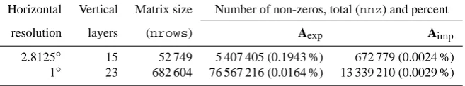
Table 1.Resolution, sizes and sparsity of one block of the explicit and implicit transport matrices for two resolutions computed with the MITgcm.

horizontal vertical matrix size number of non-zeros, total (nnz) and percent

resolution layers (nrows) Aexp Aimp

2.8125◦ 15 52 749 5 407 405 (0.1943 %) 672 779 (0.0024 %) 1◦ 23 682 604 76 567 216 (0.0164 %) 13 339 210 (0.0029 %)

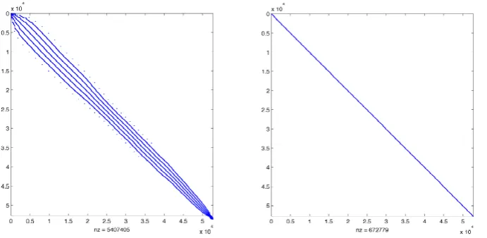
Fig. 1. One block of the explicit (left) and implicit (right) transport matricesAexp,Aimpcomputed using the MITgcm for a 2.8125◦ resolution (output of MATLAB®’sspycommand).

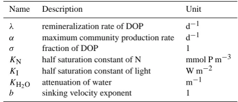
Table 2.Parameters in the N-DOP model.

Name Description Unit

λ remineralization rate of DOP d−1

α maximum community production rate d−1

σ fraction of DOP 1

KN half saturation constant of N mmol P m−3

KI half saturation constant of light W m−2

KH2O attenuation of water m−1

b sinking velocity exponent 1

Fig. 2.Compilation and linking process of the spin-up for usage on the GPU.

Fig. 1. One block of the explicit (left) and implicit (right) transport matrices Aexp,Aimpcomputed using the MITgcm for a 2.8125◦resolution

(output of MATLAB®’sspycommand).

compared to the turbulent mixing, which is a reasonable sim-plification.

The idea of the Transport Matrix Method (TMM) intro-duced in Khatiwala et al. (2005) is to compute or approxi-mate the matrices that represent an appropriate discretization ofL. This is done by running time steps of the ocean model that has produced the circulation data v, κ etc., with spe-cial, only locally non-zero initial distributions for one tracer. By varying the support of the initial distributions over the whole spatial domain, an approximation for one or several time steps can be obtained, which can be then used to build up a matrix representation ofL. A comprehensive discussion of the temporal and spatial discretization as well as the pro-cess of evaluating transport matrices, especially in combina-tion with operator splitting schemes can be found in Khati-wala et al. (2005). For our results we used twelve implicit and twelve explicit transport matrices, which represent monthly averaged diffusion and advection. The matrices are interpo-lated linearly to the corresponding discrete time step during simulation.

As a result, we obtain the following fully (temporal and spatial) discrete scheme where we now denote byyj the ap-propriately arranged vector of the values of allntracers on all spatial grid points at time stepj. In the same way, we denote byqjthe vector of the discretized source-minus-sink terms at all spatial grid points in time stepj. Using the TMM with a fixed time step-sizeτ, the time integration scheme for (Eq. 2) reads

yj+1=Aimp,j(Aexp,jyj+τqj(yj))=:ϕj(yj). (3) Here nτ is the total number of time steps and Aimp,j,Aexp,j are the implicit and explicit transport matri-ces at time stepj=0, . . . , nτ−1. The matrices are block-diagonal and sparse and depend on the used time-stepping scheme: if – as a simple and unrealistic example – the whole system were solved explicitly by an Euler step, Aimp,jwould

be the identity and Aexp,j would be the discrete counterpart ofI+τ L(κ,v, t_j). Summarizing, starting from a vectory0

of initial values, each step in the time integration scheme (Eq. 3) to solve the tracer transport equations (Eq. 1) con-sists of the evaluation of the source-minus-sink term and two matrix-vector multiplications per tracer.

Table 1 shows typical values for the sizes and sparsity of transport matrices generated by the MIT General Circulation Model (MITgcm; Marshall et al., 1997) for two spatial res-olutions, see Khatiwala et al. (2005); Piwonski and Slawig (2012). Since we deal with quadratic matrices and the spar-sity patterns remain the same throughout the whole spin-up process a characterization of the used matrices by the num-ber of rows (nrows) and the number of non-zero elements (nnz) is sufficient for our purpose. Figure 1 shows the spar-sity patterns. The matrix entries are stored as double

preci-sion values.

2.2 Computation of steady annual cycles

Computing a periodic solution of the discretized system (Eq. 3) means looking for a fixed point of the mapping 8=ϕn_τ−1◦ · · · ◦ϕ0, i.e. for a trajectory(yj)j=0,...,nτ with

ynτ =8(y0)=y0. (4)

Thus one application of the mapping8corresponds to the computation of one year model time (or model year). The time step used in our computations was 3 h, which corre-sponds (taking 360 days a year) tonτ=2880. The discretiza-tion of the biogeochemical termsqimay include shorter time steps (typically 8 per outer 3-h step).

The whole iteration to compute a steady cycle (or fixed point) now consists of a repeated application of the mapping 8:

(4)

Table 1. Resolution, sizes and sparsity of one block of the explicit and implicit transport matrices for two resolutions computed with the

MITgcm.

Horizontal Vertical Matrix size Number of non-zeros, total (nnz) and percent

resolution layers (nrows) Aexp Aimp

2.8125◦ 15 52 749 5 407 405 (0.1943 %) 672 779 (0.0024 %)

1◦ 23 682 604 76 567 216 (0.0164 %) 13 339 210 (0.0029 %)

where yl is the vector of discretized tracer after l model years, i.e.yl=yl·nτ, andnlthe total number of model years

necessary to reach a steady annual cycle. The resulting struc-ture of the spin-up is sketched in Algorithm 1.

From several computations it can be observed that after aboutnl=3000 iterations, a numerical steady solution (up to an accuracy of about 10−2in discreteL2()nnorm) is ob-tained. Thus we refer to this as a “converged steady annual cycle”. This value ofnlwas also used in (Kriest et al., 2010). The residual can be further decreased by using a higher num-bernlof model years.

2.3 Applying parallel algorithms using the PETSc library

Obviously, a parallelization of the matrix-vector multiplica-tion occurring every time step can significantly speed up the process of computing the steady annual cycle by the pseudo-time stepping (or fixed point iteration) described above. In the CPU setting (e.g. Piwonski and Slawig, 2012) the par-allelization is carried out on a multi-processor, distributed-memory architecture. In order to avoid the direct implemen-tation of MPI directives, we make use of the PETSc library. It is a collection of data structures and algorithms for the parallel solution of numerical problems and provides inter-faces (APIs) to programming languages as Fortran, C, C++, Python, and MATLAB®. Main advantages of PETSc for our application are the parallelized matrix-vector-multiplication routines and the usage of an efficient sparse matrix storage format, in our case the default PETSc format, namely the “AIJ” or “Yale sparse” or “CSR” (compressed sparse row) format.

In our original implementation, the biogeochemical part (Algorithm 1, line 4) is implemented in Fortran, whereas the remainder of the code is realized in C. There is a dif-ference with respect to the access of the tracer data that becomes important later on the GPU: for the biogeochemi-cal computations (line 4), the values of the separate tracers and also on different spatial grid points (compare Eq. 6) are needed simultaneously. In contrast, the matrix-vector prod-ucts (lines 6, 7) are executed separately for each tracer, thus allowing us to store and work with one block of the trans-port matrices only. Each matrix-vector product is computed by one call to the PETSc routineMatMult().

For the interpolation step in line 5, three other PETSc rou-tines are used (for explicit and implicit matrix separately) to compute the appropriately weighted matrices:

MatCopy(A[i_alpha], A_work, ...); MatScale(A_work, alpha);

MatAXPY(A_work, beta, A[i_beta], ...);

These three routines together compute a linear inter-polant or convex combination of two succeeding monthly averaged matrices, which are stored in the array A start-ing at indexi alpha andi beta, respectively. Thus the above lines computeA work = alpha * A[i alpha] + beta * A[i beta], which gives the desired interpo-lated matrix inA work, ifalpha, i alphaandbeta, i betaare chosen correctly with respect to the time stepj. 2.4 Ecosystem and biogeochemical model examples

We use two simple models to test the computational gain pos-sible with the GPU hardware. Each of them has two tracers (i.e. n=2 in Eq. 1 and thereafter). Source codes for both models are available at Piwonski and Slawig (2012).

The first one is a simple radioactive decay model which is uncoupled and has the autonomous source-minus-sink term q(y)=

₋

λ1y1

−λ2y2

.

The parametersλ1, λ2>0 are the decay rates of the two

radioactive elements. We chose Iodine I131withλ1≈44.88

and Caesium Cs137withλ2≈0.0331. This uncoupled model

is used in order to test the gain in CPU time for the pure matrix-vector multiplication and interpolation in the TMM.

The second model is a typical biogeochemical model, in-cluding both coupling and nonlinearities. It is based on the N-DOP model described in Parekh et al. (2005), which was also used in Kriest et al. (2010), from which we basically take the notation. The model incorporates phosphate (nutri-ents, N,y1) and dissolved organic phosphorus (DOP,y2). The

source-minus-sink term is split up into the upper, sun-lit or productive euphotic zone1 with depth z0, and the lower,

(5)

E. Siewertsen et al.: Porting marine ecosystem model spin-up to GPUs 21

Algorithm 1: Marine ecosystem spin-up using TMM

Require: Set of monthly averaged transport matrices Aimp,Aexp, initial tracer distributiony0, time stepτ Ensure : At the endyis a tracer distribution (at one point in time) of a steady annual cycle

1 y=y₀

2 repeat

3 forj=0, . . . , nτ−1 do

4 compute biogeochemical source-minus-sink terms: y˜=qj(y)

5 interpolate the monthly averaged transport matrices to the current time stepj

6 perform explicit step: yˆ=Aexp,jy 7 perform implicit step: y=A_imp_,j(yˆ+τy˜)

8 end

9 until steady annual cycle is reached

q1(y)=

₋_{f (y}

1)+λ y2 in1

(1−σ )_∂z∂F (y1)+λ y2 in2

q2(y)=

σf (y1)−λ y2 in1

−λ y2 in2

zbeing the vertical coordinate. The biological production is calculated as a function

f (y1)=α

y1

y1+KN

I

I+KI

of nutrients y1 and light I. The dependence on the

lat-ter is omitted here in the notation for brevity. The produc-tion is limited by a half saturaproduc-tion funcproduc-tion, also known as Michaelis-Menten kinetics, and a maximum production rate parameterα. Light is modeled as a portion of shortwave ra-diationISWR, which is computed as a function of latitude and

season following the astronomical formula of Paltridge and Platt (1976). The portion depends on the photo-synthetically available radiationσPAR=0.4, the ice coverσice, and the

ex-ponential attenuation of water, i.e. I=ISWRσPAR(1−σice)exp(−z KH2O).

A fraction σ of the biological production remains sus-pended in the water column as dissolved organic phospho-rus, which remineralizes with a rateλ. The remainder of the production sinks as particulate to depth where it is reminer-alized according to the empirical power–law relationship de-termined by Martin et al. (1987),

F (y1)=

_z

z0 −bz

0

Z

0

f (y1) dz. (6)

Similar modeling of biological production can be found for example in Dutkiewicz et al. (2005). Algorithm 2 sketches the implementation of the N-DOP model, whereas the model parameters are given in Table 2.

Table 2. Parameters in the N-DOP model.

K_N half saturation constant of N mmol P m−3

K_H

2O attenuation of water m

−1

3 GPU computing with CUDA

In this section we describe the basic architecture of GPUs and give an overview of some useful libraries. We concentrate on NVIDIA’s Compute Unified Device Architecture (CUDA; NVIDIA Corporation, 2012). One alternative is, for example, OpenCL (The Khronos Group, 2012).

NVIDIA, as one of the leading producers of graphic cards, has developed its own parallel architecture for executing computationally expensive code on GPUs. By exploiting the architecture of graphic cards as well as the increased memory bandwidth, it is possible to perform a far greater number of floating point operations per second (FLOPS) than on CPUs. While CPUs have about one to eight cores each with up to 4 GHz clock rate, GPUs nowadays do have a lower clock rate, but hundreds of cores which can run multiple threads simultaneously.

The basic unit of the CUDA programming model is called

kernel. A kernel is a piece of program code invoked on the

CPU host and executed on the GPU device by threads. These threads are organized in a “grid” of thread “blocks”. A call to

kernel<<<gridSize, blockSize>>>();

(6)

Algorithm 2: Computation ofy˜ =qj(y)for the N-DOP model.

Require: Tracer vectorsy, latitudeφ, ice coverσice, depthsz, layer heightsdzand parameters:λ, α, σ, KN, KH2O, KI, b

Ensure : y˜ consists of the computed sinks and sources

1 for every water columniwithni layers do

2 I=0.4∗(1−σice,i)∗ISWR(φi) // compute insolation

3 y˜=0 // zero all bio steps

4 for 8 biosteps do

5 y0=y+ ˜y // take previous steps into account

6 y˜0=0 // zero one bio step

7 for layerj=1 to min(ni,2)do // production layers

8 Ij=I∗exp(−zj KH2O)

9 fj=α∗y10,j∗Ij/(y10,j+KN)/(Ij+KI)

10 y˜0₁, j= ˜y0₁, j−fj 11 y˜0₂, j= ˜y0₂, j+σ∗fj

12 if last layer then

13 y˜0₂, j= ˜y₂0, j+(1−σ )∗fj

14 else

15 for every layerkbeneath do // approximation of dF/dz

16 if last layer then

17 y˜0₂, j= ˜y0₂, j+(1−σ )∗fj∗dzj∗(zk−1/zj)−b/dzk

18 else

19 y˜0₂, j= ˜y0₂, j+(1−σ )∗f_j∗dz_j∗((z_k−1/zj)−b−(zk/zj)−b)/dzk

20 end

21 end

22 end

23 end

24 for layerj=1 tonido // all layers

25 y˜0₁, j= ˜y₁0, j+λ∗y₂0_,j

26 y˜0₂, j= ˜y₂0, j−λ∗y₂0_,j

27 end

28 y˜ = ˜y+1/8∗ ˜y0 // scale and add to all bio steps

29 end

30 end

The GPU hardware consists of several Streaming Multi-processors (SMs). Each SM has its own buffer memory, reg-isters, and a number of cores. The cores have their own units for integer and floating-point calculation. For example, the GeForce GTX 480 used here has 15 SMs with 32 cores each, i.e. a total of 480 cores. On a core, the smallest executable unit is a “warp”, which consists of 32 threads. The total number of threads that can run simultaneously on a multi-processor is dependent on the Compute Capability (CC) of the graphics chips. For the GTX 480 the limit is 1536 threads, which results in a maximum number of concurrent threads for the entire GPU of 15×1536=23 040 (p. 159, NVIDIA Corporation, 2011).

The device memory on the GPU is divided into three types of physical and virtual portions. At first, a thread has access to its own private memory which is, depending on the CC, be-tween 16 kB and 512 kB. Secondly, threads within one block have access to a shared memory of between 16 kB and 48 kB. Finally, all threads have access to a shared global memory

whose size is limited by the total amount of memory of the GPU. In order to run kernel code on the GPU, all data must be transferred from the host memory of the CPU to the device memory on the GPU.

NVIDIA provides a compiler (nvcc) that translates C code into the CUDA Instruction Set (called PTX) and be-haves similarly to the C compiler (gcc) included in the GNU Compiler Collection (GCC). A port of the GNU debugger

gdbis also included in the CUDA toolkit.

3.1 Libraries

(7)

the GPU. For documentation and sample code we refer to (Hoberock and Bell, 2012).

The second library is Cusp (Bell and Garland, 2010), which provides data types for sparse matrices and algorithms for basic linear algebra operations on them. All data struc-tures in Cusp have a parameter that determines whether it is stored in CPU or GPU memory. Operations on the data will then take place in the respective storage area. For our ap-plication, in particular the structurecusp::csr matrix

for the CSR format and the matrix-vector multiplication rou-tinecusp::multiplythat uses the algorithm described in Bell and Garland (2008, 2009), which was specially de-veloped for GPUs, are important. Documentation and sample code can be found at (Bell and Garland, 2010).

The third library we used was the preliminary implementa-tion of PETSc for the CUDA architecture presented in Min-den et al. (2010). With the help of the Thrust and Cusp li-braries, a large part of the PETScVectorand some parts of theMatrix class have been implemented. The funda-mental problems of interaction of PETSc with the GPU have been resolved, but only the routines that were necessary for the example treated in Minden et al. (2010) have been im-plemented. Basically this “PETSc GPU” extends the built-in structures by a value that indicates in which memory the most recent data are stored. This guarantees that the correct data is available (and if necessary copied to) the memory that is cur-rently used. Here, we employed the developer PETSc library version 3.2-p5.

4 Port of the marine ecosystem simulation onto the GPU

We now describe the necessary modifications and extensions of the original program that was running on a multi-processor CPU cluster in order to perform the simulation on a GPU. Basically these modifications are extensions of PETSc GPU, modifications necessary to use the CUDA Fortran compiler for the biogeochemical model code and some routines for conversions between different data alignments.

4.1 Necessary extensions of PETSc GPU

The preliminary PETSc GPU implementation was designed to solve systems of equations, and thus not all functions nec-essary for our applications were included. To avoid any copy-ing of data between CPU and GPU storage that would have destroyed the speed-up, we had to extend the library. In our case, the three PETSc routinesMatCopy,MatScale, and

MatAXPYmentioned in Sect. 2.2 had to be modified. If using sparse matrices with PETSc and working with GPUs the PETSc wrapper function

MatCopy(Ain, Aout, ...);

accesses MatCopy SeqAIJCUSP() to copy the values from matrixAintoAout. Here, it is theoretically possible

that both matrices are either currently in the GPU memory, the CPU memory or in both. For a complete and correct implementation, it would have been necessary to cover all these cases, and accordingly select the memory the matri-ces are actually copied to. For our application it was suf-ficient to cover only the case where the matrices are both in the GPU memory, thus only this case was implemented. Therefore, an additional call toMatCUSPCopyToGPU()in

MatCopy SeqAIJCUSP()ensures that both matrices are in the GPU memory.

The PETSc routinesMatScale()andMatAXPY() im-plement typical linear algebra subproblems, which are only performed on the non-zero matrix elements. Consequently, they could be completely realized using the Cusp BLAS li-brary for the GPU.

4.2 PGI CUDA-Fortran

Many biogeochemical models are implemented in Fortran. Mostly, they are part of a software that has evolved over decades (e.g. MITgcm). Since we want to use them with GPUs without any modification to original source code, we need a Fortran compiler and the appropriate libraries. At the time of this work there was only one candidate, namely the PGI CUDA Fortran compiler (The Portland Group, 2012). It extends the language by constructs for calling kernel as well as the CUDA API functions. The syntax of a kernel call in Fortran is

call kernel<<<gridSize, blockSize>>>()

and thus similar to CUDA C++ . There are some extensions compared to CUDA C++, but also some restrictions. For de-tails we refer to the manual (The Portland Group, 2011a, p. 14).

4.3 Other extensions to the implementation on the CPU

As mentioned in Sect. 2.3, there are two different data align-ments useful for the spin-up using the TMM: one for the bio-geochemical source-minus sink terms, where all tracers of a water column are kept in a contiguous piece of memory, and another one for the multiplication with the transport matrices, where every water column of a tracer is kept together to re-duce the storage requirements for the matrices. Thus a copy-ing between these two data alignments is necessary in every step of the algorithm. For the use on the GPU, three copy-ing functions in the original code were additionally modified using the Thrust library.

4.4 The compilation process for the GPU

Here we briefly sketch the overall compilation and linking process of the resulting code for the use on the GPU. The process is visualized in Fig. 2.

(8)

24 E. Siewertsen et al.: Porting marine ecosystem model spin-up to GPUs

Table 1. Resolution, sizes and sparsity of one block of the explicit and implicit transport matrices for two resolutions computed with the

MITgcm.

horizontal vertical matrix size number of non-zeros, total (nnz) and percent resolution layers (nrows) Aexp Aimp

2.8125◦ 15 52 749 5 407 405 (0.1943 %) 672 779 (0.0024 %) 1◦ 23 682 604 76 567 216 (0.0164 %) 13 339 210 (0.0029 %)

Fig. 1. One block of the explicit (left) and implicit (right) transport matricesAexp,Aimp computed using the MITgcm for a 2.8125◦

resolution (output of MATLAB®’sspycommand).

Table 2.Parameters in the N-DOP model.

KN half saturation constant of N mmol P m−3

KH2O attenuation of water m −1

Fig. 2.Compilation and linking process of the spin-up for usage on

the GPU.

Fig. 2. Compilation and linking process of the spin-up for usage on

the GPU.

and processed to driver model.CUF by the pre-processor of the C++ compiler pgcpp. The Fortran compiler pgfortran then generates the object file

driver model.o.

The driver routine driver.CUFhas two tasks: at first the Fortran compiler requires that all functions which shall run on the GPU are marked with the device at-tribute, see The Portland Group (2011b). Since the com-piler has no ability to set default attributes for all func-tions, it is necessary to integrate them through a preprocessor macro. Therein the Fortran keyword subroutine is re-placed byattributes(device) subroutine. Sec-ondly, the driver provides support functions for the three entry points into the biogeochemical model, namely (i) the evaluation of the source-minus-sink term, (ii) the initializa-tion and (iii) deinitializainitializa-tion of the model. These three func-tions need corresponding kernels for the GPU. This approach ensures the original Fortran interface of the biogeochemical model remains unaltered.

In a second step (top left of Fig. 2) the original, unmodi-fied C code is compiled with the MPI wrapper of the GNU C compilermpicc, while CUDA extensions are translated withnvcc. Finally all object code files are linked against PGI Fortran libraries, which results in the final executable.

5 Numerical results

In this section we compare the performance of the spin-up on our CPU/GPU test hardware. We use the two models described in Sect. 2.4. A special emphasis lies on the time needed for the individual parts, namely the evaluation of the biogeochemical source minus-sink term, the matrix interpo-lation and the matrix-vector multiplication. Moreover, we

E. Siewertsen et al.: Porting marine ecosystem model spin-up to GPUs 11

Table 3.Minimum, maximum, average and standard deviation of computational time for one model year spent on the CPU and GPU. Shown are results of 100 model years, each year timed separately.BGCStepblock size: 160.

CPU GPU

model Min Max Avg StdDev Min Max Avg StdDev CPU Min:GPU Min I-Cs 159.58s 161.44s 160.19s 0.47 15.49s 15.52s 15.50s 0.002 10.30 N-DOP 621.43s 626.79s 622.14s 0.54 28.17s 28.20s 28.18s 0.003 22.06

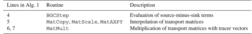
Table 4.The three main portions in every time step of the spin-up.

lines in Alg. 1 Routine Description

4 BGCStep evaluation of source-minus-sink terms 5 MatCopy,MatScale,MatAXPY interpolation of transport matrices

6, 7 MatMult multiplication of transport matrices with tracer vectors

Table 5.Mean computational time within one model year and performance gains of the individual routines depicted in Table 4.

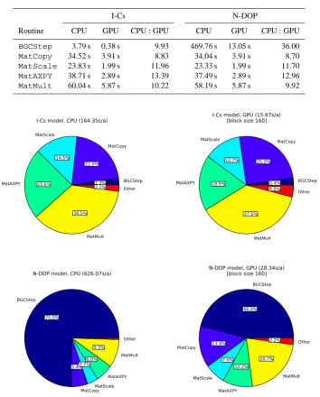
I-Cs N-DOP Routine CPU GPU CPU : GPU CPU GPU CPU : GPU

BGCStep 3.79s 0.38s 9.93 469.76s 13.05s 36.00

MatCopy 34.52s 3.91s 8.83 34.04s 3.91s 8.70

MatScale 23.83s 1.99s 11.96 23.33s 1.99s 11.70

MatAXPY 38.71s 2.89s 13.39 37.49s 2.89s 12.96

MatMult 60.04s 5.87s 10.22 58.19s 5.87s 9.92

32 128 224 320 416 512 block size 0.38 0.39 0.40 0.41 0.42 0.43 0.44 0.45 0.46 0.47

time per cycle [s]

I-Cs BGCStep

32 128 224 320 416 512 block size 12 13 14 15 16 17 18 19 20

time per cycle [s]

N-DOP BGCStep

Fig. 3.Computational time needed for the I-Cs (left) and N-DOP (right) model within one model year depending on the block size.

Fig. 3. Computational time needed for the I-Cs (left) and N-DOP

(right) model within one model year depending on the block size.

contrast the best GPU result for the N-DOP model with re-sults from three different distributed-memory architectures. 5.1 Setup

The CPU/GPU test hardware consists of two GeForce GTX 480 graphic cards and two Intel® Xeon® E5520 CPUs run-ning at 2.27 GHz. However, the following tests were per-formed only on one GPU and only on one core of the CPU. No display was connected to the graphic card and compu-tations on the GPU were performed with double precision, which is natively supported by the GTX 480. The theoretical peak performance of the GPU is at 168 GFlop s−1 and the internal bandwidth at 177 GB s−1. The performance of one core of the CPU system is at 9.08 GFlop s−1, its bandwidth at 21.2 GB s−1.

To test a specific biogeochemical model, the software is compiled with the according source code and run for 100 model years. In detail, when the executable starts the data (matrices, initial vectors, etc.) is copied into the CPU or GPU memory and 100 iterations, 2880 time steps each, are performed consecutively. In the case of a GPU run, the results are copied back to CPU memory at the end.

Thus, the whole data has to fit into the memory of the de-vice (or host). This is the case if the 2.8125◦_horizontal

res-olution is used. Here, the 1.5 GB RAM of a GTX 480 (or 40 GB of the CPU system) are enough for about 1 GB of data. However, a monthly averaged set of transport matrices based on a 1◦resolution (approximately 13 GB) is too large for the used GPU system. Such an amount of data requires a differ-ent approach (see Sect. 6). Hence, we focus on the 2.8125◦ resolution and omit profiling of data transfers between CPU and GPU memory.

When processing source codes, thempicc,mpif90and

nvcc compilers are switched to -O (i.e. optimize). For

(9)

Table 3. Minimum, maximum, average and standard deviation of computational time for one model year spent on the CPU and GPU. Shown

are results of 100 model years, each year timed separately.BGCStepblock size: 160.

CPU GPU

Model Min Max Avg StdDev Min Max Avg StdDev CPU Min:GPU Min

I-Cs 159.58 s 161.44 s 160.19 s 0.47 15.49 s 15.52 s 15.50 s 0.002 10.30

N-DOP 621.43 s 626.79 s 622.14 s 0.54 28.17 s 28.20 s 28.18 s 0.003 22.06

Table 4. The three main portions in every time step of the spin-up.

Lines in Alg. 1 Routine Description

4 BGCStep Evaluation of source-minus-sink terms

5 MatCopy,MatScale,MatAXPY Interpolation of transport matrices

6, 7 MatMult Multiplication of transport matrices with tracer vectors

5.2 Results

We start by examining the block size parameter for the For-tran kernel calls of the biogeochemical model. The block size describes the number of vertical profiles (or water columns) that are processed within a block. While the grid and block dimensions are calculated automatically, if using Thrust or Cusp for example, a suitable value for the Fortran kernel must be determined experimentally for the time being. For all tests we use just 100 model years (instead of 3000 or more needed in practice, see Sect. 2.2) to render the numerical ex-periments feasible, especially when simulating the N-DOP model on the CPU, which still takes about 17 h.

Figure 3 depicts the mean of 100 model years’ compu-tational time spent on the GPU for biogeochemical model steps depending on the block size. In both models, strong fluctuations up to 100 % occur. However, both graphs show similar occurrence of minima and maxima. We suppose this is due to the unbalanced distribution of water columns (see Sect. 6). However, the absolute minimum (I-Cs: 0.38 s, N-DOP: 12.6 s) is obtained for a block size of 160.

This value is used for the subsequent test, in which every year is timed separately. Table 3 shows the minimum, max-imum and mean of computational time for one model year spent on the CPU and GPU. The standard deviation is small on the CPU (I-Cs: 0.47, N-DOP: 0.54) and marginal on the GPU (I-Cs: 0.002, N-DOP: 0.003). However, the overall re-duction is about 10 for the simpler I-Cs model and about 22 for the more complex N-DOP model, a difference we inves-tigate further.

Thus, the next tests focus on the individual steps within the repeat-until loop of Algorithm 1, corresponding to one an-nual cycle. The invoked routines are listed in Table 4. Their individual performance gain is depicted in Table 5.

Regard-ingMatCopy,MatScale,MatAXPYandMatMult, we

see a similar relative performance gain for both models from about 9 to 13. In contrast,BGCStepshows a speed-up of

about 10 for the I-Cs model, whereas for N-DOP a ratio be-tween the CPU and GPU of 36 can be observed. In addition, in Fig. 4 we recognize that 75 % of the overall time on the CPU, which is spent for the evaluation of the N-DOP model, is sped up by this factor on the GPU. This explains the over-all ratio of 22. Note that the slightly higher average computa-tional times in Fig. 4 (compared to those in Table 3) are due to the higher granularity of profiling. Moreover, we see that the computational effort for the I-Cs model, which is just a scaling of the tracer vector, is smaller than 3 % on both ar-chitectures. Here, the overall speed up is dominated by the matrix operations.

Concerning the latter, we pickMatMult for a detailed view on performance and bandwidth and compare our results with those reported by Bell and Garland (2008). We calculate the number of floating point operations for one model year as follows:

nops=nτ∗2∗(2∗nnzexp+2∗nnzimp)≈70 GFlop,

which is the number of time steps per year times number of tracers times (explicit plus implicit) sparse matrix-vector multiplication, which is exactly twice the number of non-zeros. We consider the results from the N-DOP model and dividenopsby 58.19 s (CPU) and 5.87 s (GPU), respectively.

We obtain a performance of approximately 1.2 GFlop s−1 for the CPU and 11.9 GFlop s−1for the GPU. This is about 13 % of the theoretical peak performance of one CPU core (9.08 GFlop s−1) and about 7 % of 168 GFlop s−1, regarding the GPU. The poor performance is due to the bandwidth lim-itation, which is typical for sparse matrix-vector multiplica-tions. Following Bell and Garland (2008), we multiplynops

by 10 Byte Flop−1_{(CSR vector kernel) and relate the result}

to the computational time spent on the CPU and GPU, re-spectively. We obtain 56.8 % (12 GB s−1_{) of the theoretical}

(10)

Table 5. Mean computational time within one model year and performance gains of the individual routines depicted in Table 4.

I-Cs N-DOP

Routine CPU GPU CPU : GPU CPU GPU CPU : GPU

BGCStep 3.79 s 0.38 s 9.93 469.76 s 13.05 s 36.00

MatCopy 34.52 s 3.91 s 8.83 34.04 s 3.91 s 8.70

MatScale 23.83 s 1.99 s 11.96 23.33 s 1.99 s 11.70

MatAXPY 38.71 s 2.89 s 13.39 37.49 s 2.89 s 12.96

MatMult 60.04 s 5.87 s 10.22 58.19 s 5.87 s 9.92

12 E. Siewertsen et al.: Porting marine ecosystem model spin-up to GPUs

BGCStep 2.3%

MatCopy

21.0% MatScale

14.5%

MatAXPY 23.6%

MatMult 36.5%

Other 2.1%

I-Cs model, CPU (164.35s/a)

BGCStep 2.4%

MatCopy

25.0% MatScale

12.7%

MatAXPY 18.5%

MatMult 37.5%

Other 4.0%

I-Cs model, GPU (15.67s/a) [block size 160]

BGCStep

75.0%

MatCopy 5.4%

MatScale 3.7%

MatAXPY 6.0% MatMult

9.3%

Other

N-DOP model, CPU (626.07s/a)

BGCStep

46.0%

MatCopy 13.8%

MatScale 7.0%

MatAXPY 10.2%

MatMult 20.7%

Other 2.2%

N-DOP model, GPU (28.34s/a) [block size 160]

Fig. 4.Fraction of computational time needed for the individual parts in one year of the spin-up (Algorithm 1 and Table 4) for the I-Cs (top) and the N-DOP (bottom) model on the CPU (left) and GPU (right).

Fig. 4. Fraction of computational time needed for the individual parts in one year of the spin-up (Algorithm 1 and Table 4) for the I-Cs (top)

and the N-DOP (bottom) model on the CPU (left) and GPU (right).

These figures in turn are satisfying and confirm a good performance of the CSR vector kernel used by MatMult. However, they also show that a sparse matrix-vector mul-tiplication on a GTX 480, which is two generations ahead of the GTX 280 used by Bell and Garland (2008), is only slightly faster. Here, we refer to the 10 GFlop s−1, achieved by the GTX 280 for “unstructured” matrices, compared to the 11.9 GFlop s−1achieved by the GTX 480 for the trans-port matrices. This is obviously due to the only slightly in-creased memory bandwidth from 141.7 GB s−1 (GTX 280) to 177 GB s−1(GTX 480).

Nevertheless, motivated by the overall speed up, we per-form simulations of the N-DOP model on three different CPU clusters and put them in relation to the best performance on the GPU as a last comparison. Figure 5 shows that a GTX 480 can compete with approximately 56 Barcelona, 28 West-mere, and 17 Gainestown processors.

6 Conclusions

(11)

E. Siewertsen et al.: Porting marine ecosystem model spin-up to GPUs

13

10 17 20 28 30 40 50 56 60 processor count

28 50 100 150

time per cycle [s]

Simulation of one cycle (N-DOP, 2.8125°, 2880 time steps) 2.10 GHz AMD Barcelona (rzcluster) 2.67 GHz Intel Westmere (rzcluster) 2.93 GHz Intel Gainestown (HLRN) GeForce GTX 480

Fig. 5.Comparison between CPU cluster and the used GPU for one model year for the N-DOP model, (“rzcluster” refers to the Kiel

University cluster, “HLRN” to the cluster of theNorth-German

Su-percomputing Alliance).

Fig. 5. Comparison between CPU cluster and the used GPU for one

model year for the N-DOP model, (“rzcluster” refers to the Kiel University cluster, “HLRN” to the cluster of the North-German

Su-percomputing Alliance).

extensions to the used libraries were necessary. This work required knowledge in the computing architecture of the used CUDA programming framework and the PETSc, Thrust and Cusp libraries. In order to compile Fortran code for the GPU, a commercial compiler was necessary.

Concerning the computational gain of the used biogeo-chemical models, we were surprised by the good perfor-mance of the N-DOP implementation. Here, we can only speculate about the reasons and see a need for a more detailed investigation. Considering the complexity of Algorithm 2, however, such an effort was out of the scope of this work. We thus reported only results here.

RegardingMatMult, we observed a similar good utiliza-tion of memory bandwidth by the CSR vector kernel for transport matrices as reported by Bell and Garland (2008) for “unstructured” matrices. Moreover, all matrix operations showed a satisfactory performance gain.

Our results motivate us to investigate other biogeochemi-cal models and to get to the bottom of the significantly higher speed-up of the N-DOP model compared to other operations. Additionally, we are eager to prepare the code for usage with multiple GPUs and/or techniques of simultaneous copying and computing.

Acknowledgements. The GPU computations were performed with

kind permission and support of the Research Group for Com-munication Systems at Christian-Albrechts-Universit¨at of Kiel, Institute for Computer Science. The access to the HLRN computing facility was kindly provided by the group Marine Biogeochemical Modelling at IfM GEOMAR, Kiel, Germany. Moreover, the authors would like to thank two anonymous reviewers for their very helpful comments.

Edited by: D. Ham

References

Balay, S., Gropp, W. D., McInnes, L. C., and Smith, B. F.: Efficient Management of Parallelism in Object Oriented Numerical Soft-ware Libraries, in: Modern SoftSoft-ware Tools in Scientific Comput-ing, edited by: Arge, E., Bruaset, A. M., and Langtangen, H. P., Birkh¨auser Press, 163–202, 1997.

Balay, S., Buschelman, K., Gropp, W. D., Kaushik, D., Knepley, M. G., McInnes, L. C., Smith, B. F., and Zhang, H.: PETSc Web page, available at: http://www.mcs.anl.gov/petsc (last access: 7 January 2013), 2012.

Bell, N. and Garland, M.: Efficient sparse matrix-vector multiplica-tion on CUDA, Technical Report NVR-2008-04, NVIDIA Cor-poration, 2008.

Bell, N. and Garland, M.: Implementing sparse matrix-vector mul-tiplication on throughput-oriented processors, in: SC ’09: Pro-ceedings of the Conference on High Performance Computing Networking, Storage and Analysis, New York 2009, ACM, 1– 11, 2009.

Bell, N. and Garland, M.: Cusp: Generic Parallel Algorithms for Sparse Matrix and Graph Computations, available at: http: //cusp-library.googlecode.com (last access: 7 January 2013), 2010.

Bell, N. and Hoberock, J.: Thrust: A Producivity-Oriented Library for CUDA, GPU Computing Gems Jade Edition, 2011. Dutkiewicz, S., Follows, M., and Parekh, P.: Interactions of the iron

and phosphorus cycles: A three-dimensional model study, Global Biogeochem. Cy., 19, 1–22, 2005.

Hanappe, P., Beuriv´e, A., Laguzet, F., Steels, L., Bellouin, N., Boucher, O., Yamazaki, Y. H., Aina, T., and Allen, M.: FA-MOUS, faster: using parallel computing techniques to acceler-ate the FAMOUS/HadCM3 climacceler-ate model with a focus on the radiative transfer algorithm, Geosci. Model Dev., 4, 835–844, doi:10.5194/gmd-4-835-2011, 2011.

Hoberock, J. and Bell, N.: Thrust, available at: http://thrust.github. com (last access: 7 January 2013), 2012.

Horn, S.: ASAMgpu V1.0 – a moist fully compressible atmospheric model using graphics processing units (GPUs), Geosci. Model Dev., 5, 345–353, doi:10.5194/gmd-5-345-2012, 2012.

Khatiwala, S.: A computational framework for simulation of bio-geochemical tracers in the ocean, Global Biogeochem. Cy., 21, GB3001, doi:10.1029/2007GB002923, 2007.

Khatiwala, S., Visbeck, M., and Cane, M.: Accelerated simulation of passive tracers in ocean circulation models, Ocean Modell., 9, 51–69, 2005.

Kriest, I., Khatiwala, S., and Oschlies, A.: Towards an as-sessment of simple global marine biogeochemical mod-els of different complexity, Prog. Oceanogr., 86, 337–360, doi:10.1016/j.pocean.2010.05.002, 2010.

Marshall, J., Adcroft, A., Hill, C., Perelman, L., and Heisey, C.: A finite-volume, incompressible Navier Stokes model for studies of the ocean on parallel computers, J. Geophys. Res., 102, 5753– 5766, 1997.

Martin, J. H., Knauer, G. A., Karl, D. M., and Broenkow, W. W.: VERTEX: carbon cycling in the northeast Pacific, Deep Sea Res. Part A, 34, 267–285, 1987.

(12)

NVIDIA Corporation: CUDA C Programming Guide, available at: http://developer.download.nvidia.com/compute/DevZone/docs/ html/C/doc/CUDA C Programming Guide.pdf (last access: 7 January 2013), 2011.

NVIDIA Corporation: CUDA, available at: http://www.nvidia.com/ object/cuda home new.html (last access: 7 January 2013), 2012. Paltridge, G. W. and Platt, C. M. R.: Radiative Processes in

Meteo-rology and Climatology, Elsevier, New York, 1976.

Parekh, P., Follows, M. J., and Boyle, E. A.: Decoupling iron and phosphate in the global ocean, Global Biogeochem. Cy., 19, GB2020, doi:10.1029/2004GB002280, 2005.

Piwonski, J. and Slawig, T.: Metos3D: A Marine Ecosystem Toolkit for Optimization and Simulation, CAU Kiel, Institut f¨ur Infor-matik, available at: https://github.com/metos3d (last access: 7 January 2013), 2012.

The Khronos Group: OpenCL – The open standard for parallel pro-gramming of heterogeneous systems, available at: http://www. khronos.org/opencl/ (last access: 7 January 2013), 2012. The Portland Group: PGI Fortran Compiler Reference Manual,

available at: http://www.pgroup.com/doc/pgiref.pdf (last access: 7 January 2013), 2011a.

The Portland Group: CUDA Fortran Programming Guide and Ref-erence, available at: http://www.pgroup.com/doc/pgicudafortug. pdf (last access: 7 January 2013), 2011b.

The Portland Group: PGI CUDA-Fortran Compiler, available at: http://www.pgroup.com/resources/cudafortran.htm (last access: 7 January 2013), 2012.