Effects of Vertical Temperature Gradient on Heavy Gas Dispersion in Build up Area

(1)

26

Effects of Vertical Temperature Gradient on Heavy Gas

Dispersion in Build up Area

E. Kashi1_{, F. Shahraki}2∗_{, D. Rashtchian}3_{, A. Behzadmehr}4

1,2- Department of Chemical Engineering, University of Sistan and Baluchestan, Zahedan, Iran. 3- Department of Chemical and Petroleum Engineering, Sharif University of Technology, Tehran, Iran.

4- Department of Mechanical Engineering, University of Sistan and Baluchestan, Zahedan, Iran.

Abstract

Dispersion of heavy gases is considered to be more hazardous than the passive ones because it takes place more slowly. When the gas is accidentally released at ground level or where there are many obstacles in the area it is considered to be a heavy gas. In this paper, based on the extensive experimental work of McQuid and Hanna, the model was tested against two types of experiments: A simple experiment “Thorney Island” and a complex experiment “Kit Fox” in order to validate CFD code. In order to accomplish this validation the multiphase approach was employed. Also, the vertical temperature gradient in the atmosphere was investigated. The investigation of wind speed was done taking factors such as time, height and direction into consideration. In order to reduce the number of elements in the computational domain, a combination of 2D and 3D geometry was utilized. The results showed that the wind inlet correction, as well as the temperature gradient, had a significant influence on gas concentration records.

Keywords: Heavy gas dispersion, Temperature gradient, Complex train,CFD

∗ Corresponding author: [email protected] 1- Introduction

In today’s modern industry, large quantities of hazardous toxic substances are produced, stored or transported. Many of these substances are gases that form clouds heavier than air when accidentally released into the atmosphere. These gases may have a density greater than that of the air for several reasons including the high molecular weight (like

chlorine), low release temperature (like liquefied natural gas), high storage pressure (for example a failure of the container of ammonia and subsequent formation of aerosol) or chemical reactions of the released substances with water vapor in the atmosphere (the polymerization of hydrogen fluoride) [1].

(2)

Iranian Journal of Chemical Engineering, Vol. 6, No. 3 27 buoyancy that affects and modifies its

behavior when compared to a positively or neutrally buoyant cloud. These effects include the additional gravity driven flow, wind shear at the heavy gas cloud interfaces, turbulence dumping, and inertia of the released material. Some special models have been developed to describe the heavy gas clouds dispersion in the atmospheric air known as heavy gas dispersion models or dense gas dispersion models [2].

These models include empirical, intermediate and fluid dynamic models. The empirical and intermediate models are important components of emergency response systems and valuable tools for environmental impact assessment and risk assessment. The fluid dynamics models are usually used as a research tool to better understand the properties of the heavy gas.

Computational fluid dynamics allows the simulation of complex physical processes describing heat and mass transport phenomena with fully developed mathematical models. Specific models incorporated in CFD codes predict the turbulent mixing between gas molecules and air particles. This mostly happens in cavity regions in the flow field (building wakes), which may result in the entrapment of escaping gas at low heights for relatively long periods of time with increased health effects [3].

Dense gas dispersion modeling in the obstacle area, because of sensitivity to various parameters and conditions, is very complicated and is an interest in many researches, both in safety and environmental fields. Some of the recent CFD works on gas dispersion modeling have focused on

obstacle effects on gas concentration phenomena [4-9], while others studied the effects of heat transfer on LNG spills [10-12]. In this paper, numerical simulation of the Thorney Island trials and Kit Fox field experiments were performed using ANSYS CFX 11 code [13]. In this paper, CFD code is used to investigate some of the essential parameters in dense gas dispersion modeling (e.g. obstacle effects, wind profile, atmos-pheric stability and CFD parameters like mesh type and size, turbulence models, various boundary conditions) in the obstacle area.

The special studies which have been taken in to consideration in this paper are:

a) Using and testing multiphase approach instead of the additional variable model and multicomponent model for dense gas dispersion modeling.

b) A new method for wind inlet at the inlet boundary condition is used, which is three dimensional and time-dependent wind speed, instead of the usual wind profile, and is included in the model.

c) A buoyancy model (Boussinesq), instead of atmospheric stability models, is used and its effects have been studied.

d) Hybrid 2D and 3D geometry is used in order to reduce the number of meshes and computational time.

2- Field experiments

(3)

28 Iranian Journal of Chemical Engineering, Vol. 6, No. 3

of complex buildings where the flow is relatively simple and well-defined. By using this procedure any problems within the code, can be more easily identified and resolved. So, at first, the Thorney Island experiment has been simulated as a simple case and then the Kit Fox experiment is considered as a more complex experiment. Field gas dispersion experiments are very expensive and set up in some large projects, so it is not the aim of this work and, consequently, we had to use standard experiments by permission.

2.1. Thorney island experiment

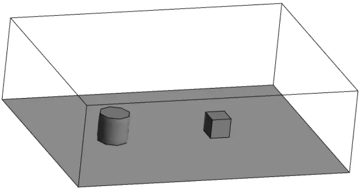
The Thorney Island Heavy Gas Dispersion Trials were organized by the Health & Safety Executive and their related detailed information has been given by McQuaid and Roebuck [14]. This experiment was investigated by Hall [15] and Sklavounos and Rigas [3]. Fig. 1 shows the schematic of trial

no. 26 of phase two which is considered in this simulation.

2.2. Kit Fox field experiment

A joint field experiment (named "Kit Fox") was conducted in August and September, 1995, at the Frenchman Flat area of the Nevada Test Site (NTS). The field operations, described in the WRI report [16], were carried out by Western Research Institute (WRI) and Desert Research Institute (DRI). There were 52 independent Kit Fox data trials, with about 2/3 for “puff” or ”finite duration” 20s releases, and about 1/3 for “continuous plume” 120-450s releases. A summary of the major characteristics of each of the 52 tests is given by Hanna and Chang [17, 18]. Fig. 2 shows the plot plan of the Kit Fox experiment. In this paper trial 3-7 (trial 3, release 7; an instantaneous release) are implemented for simulation purposes.

(4)

Iranian Journal of Chemical Engineering, Vol. 6, No. 3 29 Figure 2. Plot plan of the Kit Fox dispersion grid including meteorological towers, concentration monitoring arcs, gas source, Equivalent Roughness Pattern (ERP), and Uniform Roughness Array (URA).

3. Mathematical formulation

Gas dispersion in atmosphere can be studied in different methods using CFD code. These methods include studying a flow with an additional variable, a flow with multi-component fluid and a multiphase flow. Using additional variables can help in modeling the transport of a passive material in the fluid flow like smoke in the air. The presence of an additional variable does not affect the fluid flow, even though some fluid properties may be defined to be dependent on additional variables. In multicomponent flow method it is assumed that different components of a fluid are mixed together at molecular level sharing the same mean velocity, pressure and temperature fields. Also, in this approach mass transfer is considered to take place by convection and

diffusion. In more complex situations where different components are mixed on larger scales and with separate velocity and temperature fields, multiphase flow method is used.

In this paper, in order to model dense gas dispersion the multiphase flow method was employed. ANSYS CFX was used as a computational code for simulation purposes. In ANSYS CFX the equations of momentum, mass transfer, heat transfer, buoyancy and the turbulence model for homogeneous multiphase flow are supposed to be solved using the finite volume method.

4. Simulations and results 4.1. Thorney island case

(5)

meshing geometry. Using embedded meshing techniques, cells are concentrated around the initial position of the gas cloud in order to capture the detailed shear and entrainment effects at the edge of the gas column. In addition, a fine resolution was used vertically from the ground up to a height of about 2m. In this case 10 inflation layers were used with a first layer thickness of 0.01m. Cells close to the cube were also concentrated to help resolve the interaction problems between the cloud and obstacle. Maximum distance of meshes near the initial gas cloud is 0.5m and the normal maximum distance is 2m.

Computational grids consist of 331179 cells. Since the purpose of the study was to compute concentration values in time, the problem was solved in transient form. Total simulation time was 200s with relatively short time steps (1s). The convergence criterion was the RMS (residual of root mean

square) that was considered to be equal to or less than 10−4. Transient runs needed 3–8 iterations per time step to reach the desirable residual value.

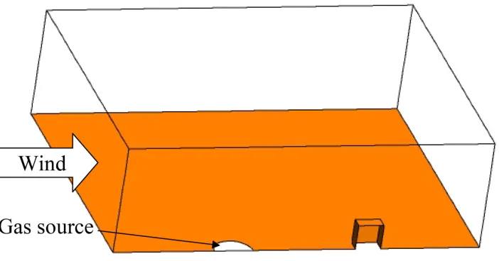
In order to reduce the number of meshes and then decrease the computing time a symmetry plane was used. The model geometry is shown in Fig. 3. The extent of the domain was 130m in the x-direction, 100m in the y-direction and 40m in the z-direction.

As mentioned earlier, R-12 and Nitrogen were used in the Thorney Island experiment. Therefore these two gases are considered in addition to air in the domain. Since Thorney Island trials were conducted at a neutral atmospheric condition and temperature data are not available we do not consider heat transfer models, and actually the equation of energy is not taken into account. Assuming there might be turbulence in the domain the standard k-ε model was used.

(6)

Iranian Journal of Chemical Engineering, Vol. 6, No. 3 31 4.1.1. Boundary conditions

Taking into consideration the computational domains shown in Fig. 3, the boundary conditions set for the wind profile and gas inflow are demonstrated below.

4.1.1.1. Gas inlet

Approximately 2000m3 of Freon 12/nitrogen mixture was released into the atmosphere instantaneously at Thorney Island no. 26. In order to set the inflow boundary condition for the transient problem, released mixture mass inflow rate (Qi) was given through a

properly adapted step function:

(

)(

)

⎥ ⎦ ⎤ ⎢ ⎣ ⎡₋ − − × = ₂ 0 1 0 t t t t t step m

Qi i (1)

where mi is equal to 4780 kg s-1.

The gas was released from the ground level source to the domain for 1s, elevating to a 13m height. After 1s a cylindrical cloud was formed. This condition was the same as the experimental condition and positively affected the simulation process.

4.1.1.2. Wind inlet

Wind speed is one of the most significant parameters in the problem definition procedure, since it determines how quickly emitted gas will be diluted by passing volumes of air. The corresponding boundary condition should take into account the reduction of wind speed value near the ground level due to the frictional effects. If wind speed at a fixed height is known (typical reference height 10m), then the wind velocity profile may be given through a power low correlation [19]:

λ ⎟⎟ ⎠ ⎞ ⎜⎜ ⎝ ⎛ × = 0 0 Z Z u

uz (2)

where λ is a dimensionless parameter whose value depends upon the atmospheric stability category and surface roughness (Z0).

Regarding the trial 26, the value of Z0 is

0.005m; λ is 0.07and u0is 1.9m/s.

In addition to the above mentioned boundary conditions, the ground and the building surfaces were defined as fixed stable walls, where according to the no-slip condition the fluid velocity is equal to zero. As mentioned earlier, half of the domain is considered because of symmetry, while the remaining surfaces of the domain were specified via a relative pressure value that was set equal to zero (opening condition).

4.1.2. Results

In Fig. 4 the predicted concentration is compared with the experimental concentra-tion measured on the front face of the building at the height of 6.4m. These results show that this model can be used for the Kit Fox experiment (as a complex experiment). It is seen that the simulation results are in good agreement with the experimental data and it can be hoped that good results from the simulation of the complex experiment will be seen.

4.2. Kit Fox case

(7)

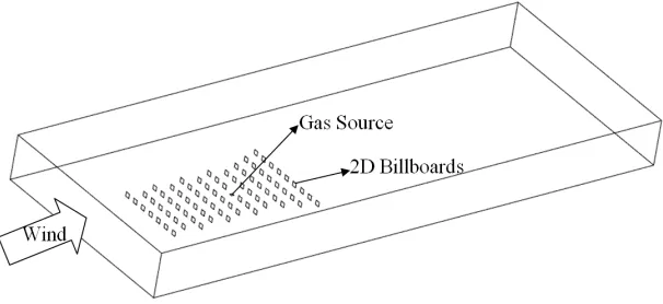
thickness of the obstacles is eliminated and as a result even the smallest mesh can be greater than the billboard thickness. The model geometry is shown in Fig. 5.

Using line control techniques, cells were concentrated around the obstacles area. Also, a fine resolution was implemented vertically from the ground up to a height of about 1m. In this study 20 inflation layers were used. The thickness of the first layer was determined at the beginning. Since the CFX

code used the wall function in its simulation and the near wall meshes are very important, the determination of the first layer was done using y+ means. This can help attain the best results from the CFD code. Maximum distance of meshes in the area around the obstacles is 0.5m and the normal maximum distance is 2m. Fig. 6 shows the refinement of meshes near the surface and around the obstacles. The fine meshes covered a volume of 6*50*100m (height*latitude* longitude)

Figure 4. Gas concentration vs. time for Thorney Island experiment (trial no. 26), front face of the building at height 6.4m.

(8)

Iranian Journal of Chemical Engineering, Vol. 6, No. 3 33 Figure 6. Surface mesh of trial 3-7 from Kit Fox experiments

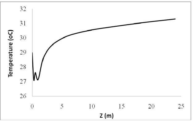
Computational grids consist of 1716184 cells. The problem was solved in transient form. Total time for simulation was set to be 250s with relatively short time steps (0.25s). The following hypotheses are considered. The fluid under consideration is a mixture of air and CO2. The air temperature was not

fixed and it varied vertically (in Z direction, see Fig. 7). Therefore the computation was carried out using thermal energy, and because of the low temperature gradient, the Boussinesq buoyancy model was used. Since the flow was assumed to be turbulent the standard k-ε model was used.

(9)

4.2.1. Boundary conditions 4.2.1.1. Gas inlet

In trial 3-7 of the Kit Fox field experiment, carbon dioxide was released instantaneously into the atmosphere with a 3.65kg/s rate and for about 20s. In order to set the inflow boundary condition, as in the Thorney Island case, the mass inflow rate of the gas from the surface level was specified (mi=3.65kg/s,

t1=50s). In order to have a fully developed

flow in the domain, the gas was released after 50s. Since the gas was released at the ground level and during the experiment the ground surface temperature was 29°C, the gas temperature was set to be 29°C in the simulation.

4.2.1.2. Wind inlet

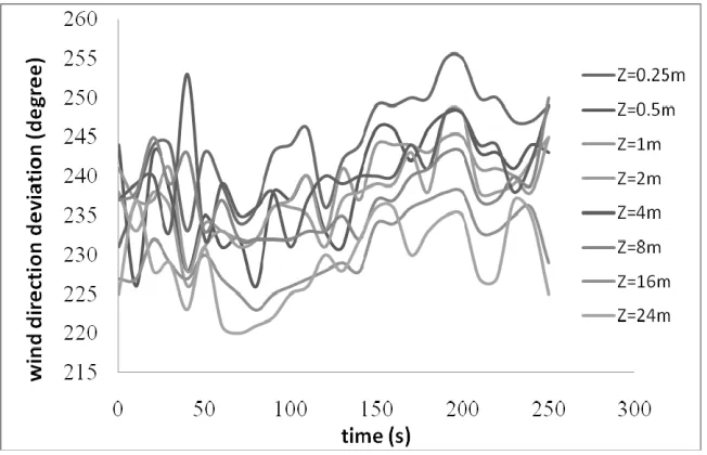
When there is low wind speed condition, wind direction can vary considerably within small periods of time. Low wind speeds are

associated with a phenomenon called meander which is a horizontal oscillation of the local atmosphere. As the wind velocity decreases below a certain threshold, it is no longer possible to define a mean wind direction (see Fig. 8). These oscillations are independent of atmospheric stability or topography and are related to the equilibrium between the coriolis force and the pressure gradient [20]. Accordingly, in order to get better results there was no use of correlation in this simulation. The EPA tower wind data (see section 3.2) was directly used as the wind inlet boundary condition. This procedure can be useful in defining the wind speed and its direction any time and in any height. The average values of wind speed and its direction are given in Table 1. Cartesian velocity component was used for adding wind direction:

(10)

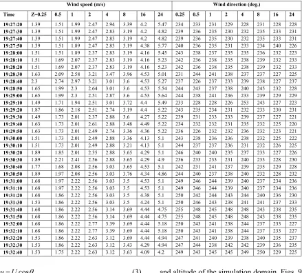
Iranian Journal of Chemical Engineering, Vol. 6, No. 3 35 Table 1. Wind speed and direction deviation with time and height in EPA tower, in trial 3-7 of Kit Fox experiments

Wind speed (m/s) Wind direction (deg.)

Time Z=0.25 0.5 1 2 4 8 16 24 0.25 0.5 1 2 4 8 16 24

19:27:20 1.39 1.51 1.99 2.47 2.94 3.39 4.2 5.47 234 233 231 229 228 231 228 228

19:27:30 1.39 1.51 1.99 2.47 2.83 3.19 4.2 4.82 239 236 235 230 232 235 233 231

19:27:40 1.39 1.51 1.99 2.47 2.83 3.19 4.2 4.82 239 236 235 230 232 235 233 231

19:27:50 1.39 1.51 1.89 2.47 2.83 3.19 4.38 5.77 240 236 235 231 233 234 240 226

19:28:00 1.51 1.51 1.89 2.37 2.83 3.19 4.16 5.45 243 238 237 235 235 236 232 223

19:28:10 1.51 1.69 2.07 2.37 2.83 3.19 4.16 5.23 242 236 238 235 238 239 232 233

19:28:20 1.51 1.69 2.07 2.37 2.83 3.19 4.16 5.23 242 236 238 235 238 239 232 233

19:28:30 1.63 2.09 2.58 3.21 3.47 3.96 4.53 5.01 231 244 241 238 237 237 227 225

19:28:40 2.3 2.74 2.97 3.21 3.01 3.6 4.53 5.27 237 226 237 233 239 238 227 237

19:28:50 1.65 1.99 2.3 2.64 3.01 3.6 4.53 5.54 244 243 237 238 240 245 232 228

19:29:00 1.65 1.99 2.3 2.51 2.87 3.6 4.53 5.64 244 238 241 236 233 239 229 229

19:29:10 1.49 1.71 1.94 2.51 3.01 3.72 4.4 5.49 233 228 228 226 253 243 227 223

19:29:20 1.87 1.86 2.18 2.51 2.74 3.19 4.4 5.22 243 235 234 231 232 233 230 231

19:29:30 1.49 1.73 2.01 2.37 2.88 3.6 4.27 5.22 239 231 233 233 239 237 227 221

19:29:40 1.63 1.73 2.01 2.61 2.88 3.48 4.49 5.22 234 232 232 231 235 232 225 220

19:29:50 1.63 1.73 2.01 2.49 2.74 3.36 4.36 5.22 236 226 232 232 236 232 223 221

19:30:00 1.51 1.73 2.01 2.49 2.88 3.36 4.13 5.1 243 238 236 236 238 232 225 222

19:30:10 1.51 1.73 2.01 2.49 2.88 3.21 4.13 5.1 244 237 237 236 231 232 226 225

19:30:20 1.89 1.85 2.01 2.35 2.88 3.65 4.29 5.1 246 240 240 235 237 233 227 226

19:30:30 1.89 2.21 2.41 2.56 2.88 3.65 4.29 4.9 236 233 233 231 240 233 228 230

19:30:40 1.77 1.68 2.08 2.56 3.03 3.65 4.53 5.1 242 231 241 237 239 235 229 228

19:30:50 1.89 1.97 2.08 2.56 3.03 3.76 4.34 4.86 244 240 237 238 240 232 228 232

19:31:00 1.68 1.97 2.22 2.56 3.03 3.5 4.53 5.1 249 246 244 239 240 237 234 236

19:31:10 1.68 1.97 2.22 2.56 3.03 3.5 4.53 5.1 249 246 244 239 240 237 234 236

19:31:20 1.68 1.86 2.22 2.56 3.03 3.5 4.38 5.1 250 242 244 243 244 240 236 230

19:31:30 1.53 1.86 2.22 2.56 3.03 3.5 4.24 5.1 250 246 243 238 241 241 237 233

19:31:40 1.68 1.86 2.22 2.56 3.14 3.69 4.44 4.75 255 248 245 248 248 243 238 235

19:31:50 1.68 1.86 2.22 2.56 3.14 3.69 4.44 4.75 255 248 245 248 248 243 238 235

19:32:00 1.68 1.86 2.22 2.77 3.39 3.69 4.44 5.18 250 243 241 238 244 237 233 227

19:32:10 1.68 1.86 2.22 2.77 3.39 3.69 4.44 5.18 250 243 241 238 244 237 233 227

19:32:20 1.53 1.86 2.22 2.63 3.12 3.69 4.44 4.94 247 241 240 239 238 240 235 237

19:32:30 1.53 1.86 2.22 2.63 3.12 3.43 4.29 4.94 247 244 238 242 242 239 236 235

19:32:40 1.53 1.75 2.22 2.63 3.12 3.63 4.09 4.2 249 243 245 245 249 250 229 225

θ

cos

U

u= (3)

θ

ν =Usin (4)

0 =

w (5)

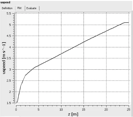
where θ is a deviation of wind direction. To consider the time variation of the wind speed and its direction in time, in the simulation step function. In this way, in comparison to the existing wind profiles like the logarithmic profile, the wind velocity was more accurately modeled (see Figs. 9 and 10). Also, there is no need to extend the longitude

and altitude of the simulation domain. Figs. 9 and 10 show wind speed dependency on time and height at x direction. Since in this trial the normal wind direction has deviations from normal x line, both the front and right sides of the domain were defined as the wind inlets. u component at the front side and the v

(11)

Figure 9. u component of wind speed at the height of 2m in EPA tower location that was included in the simulation

Figure 10. u component of wind speed from 10 to 20 seconds after gas release in EPA tower location that was included in the simulation

4.2.1.3. Surface roughness

The surface roughness length, Zo, is a

measure of the amount of mechanical mixing introduced by the surface roughness elements. The appropriate wind profile

formula for nearly neutral conditions is:

⎟⎟ ⎠ ⎞ ⎜⎜ ⎝ ⎛ =

0 * ln

1

Z Z u

u

(12)

Iranian Journal of Chemical Engineering, Vol. 6, No. 3 37 where κ is the von Karman constant

(assumed to be equal to 0.4) and u* is the friction velocity. Z0 can be obtained from

these relations [21]:

* 0

u

Z =β ν (7)

4 . 3 ln ln * − = ν

β eu (8)

where e is the real roughness height, and ν is the kinematic viscosity. As a rough rule of thumb, Z0 is equal to about 0.1 times the

average height of the roughness elements [22]. In this simulation the ground surface was defined as a rough wall with Z0 equal to

0.01m.

As mentioned earlier, the ground surface temperature was 29°C at the time of the experiment. Therefore the surface temperature was set to be 29°C.

4.2.2. Results and discussion

Since the average velocity of air before gas release is 2.7m/s and the distance between the front surface of the domain (wind boundary condition) and gas source is about 90m, the air particles need at least 50 seconds to reach the source. For the simulation, since the gas was discharged from the source 50s after introducing the air into the domain, the velocity values of the air were taken into consideration 50s before the gas release. This helped maximize the effects of wind speed variations on gas dispersion in the domain.

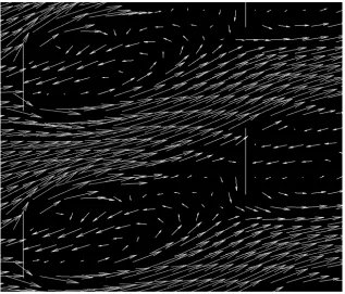
In order to investigate the grid performance, the problem was solved in a steady state condition. Flow vectors were studied on

(13)

Figure 11. Flow vectors on the 1m elevated plane

(14)

Iranian Journal of Chemical Engineering, Vol. 6, No. 3 39 (a)

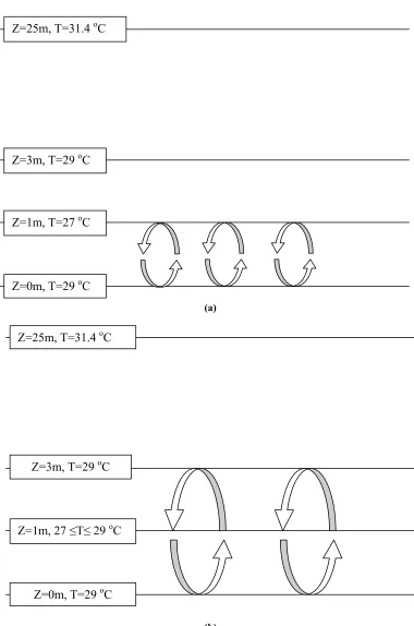
(b)

Figure 13. Flow recycles in the obstacle area Z=25m, T=31.4 oC

Z=3m, T=29 oC

Z=1m, 27 ≤T≤ 29 oC

Z=0m, T=29 oC Z=25m, T=31.4 oC

Z=3m, T=29 oC

Z=1m, T=27 oC

(15)

For comparison purposes this simulation was also carried out with logarithmic wind profile (without heat transfer model). In Figs. 14-17 gas concentration histories were compared taking the presence and absence of the heat transfer model and logarithmic wind profile conditions into consideration with the values recorded on arc one (25m far from the source) at heights of 0.3m, 0.6m, 1.2m and arc two (50m far from the source) at the height of 0.5m. Unfortunately, as these figures show, the concentration histories are better matched with the experimental results when the heat transfer model is excluded. When the heat transfer model is included, the vertical fluctuation is produced in the flow pattern and consequently the gas dispersion

is more complex and its concentration does not match very well with the experimental results.

Comparing the vertical velocity component that is produced by heat transfer between the surface and adjacent air in cases with and without the heat transfer model (Fig.18), we can see that in the second case vertical velocity does not exist, and therefore, if we eliminate the heat transfer model, actually this vertical velocity will be eliminated and gas dispersion is carried out in z direction only by molecular diffusion. This figure also shows the negative speed of the flow in the z direction near the surface. These findings illustrate the advantages of using heat transfer model.

(16)

Iranian Journal of Chemical Engineering, Vol. 6, No. 3 41 Figure 15. Comparison of experimental and computational results in Kit Fox experiment

(trial 3-7) on arc one, at height 0.6m.

(17)

Figure 17. Comparison of experimental and computational results in Kit Fox experiment (trial 3-7) on arc two, at height 0.5m.

(18)

Iranian Journal of Chemical Engineering, Vol. 6, No. 3 43 When the dense gas is released, contrary to

the passive gas, it moves upward and flows like a liquid. This phenomenon is clearly shown in Fig. 19. Once the dispersion of the gas is over the gases obstructed at the rear of the obstacles act like secondary sources and therefore the gas dispersion process will continue for longer periods of time. Contrary to the old gas dispersion models, the CFD models can properly show this phenomenon. CFD postprocessor also can help figure out the volumes of clouds of the flammable gases that have concentrations higher than their related LFL. The weight of the gas cloud can also be obtained. This can be used for calculating the power of an explosion.

5- Conclusion

Computational simulations of atmospheric dispersion of gas around both an isolated cubical obstacle and an array of obstacles were conducted using the code CFX11. The model was validated using the results of Thorney Island and Kit Fox experiments.

The fluctuations of wind speed and its direction are the most important factors in an accidental gas release. By including experimental wind speed and direction data at different times and elevations in CFD code, the concentration results can be predicted more carefully. In addition, the near wall mesh size is an important parameter that can affect gas dispersion. Using y+_{means at the mesh generation stage}

helped in achieving acceptable and desirable results more easily. The vertical temperature gradient is an important phenomenon in gas dispersion modeling that has been shown by stability class in old models. In CFD models, temperature gradient should be considered in the simulation as a boundary condition using profiles or raw experimental data.

6- Acknowledgement

The authors wish to express their deep gratitude for providing Kit Fox field experiment data to Dr. Joseph Chang from George Mason University.

(19)

References

1. Markiewicz, M., Models and techniques for health and environmental hazard assessment and management. Center of Excellence Management of Health and Environmental Hazard, Otwock, Swierk (2006).

2. Lees, F. P., Loss prevention in the process industries hazard identification, Assessment and Control, Second edition, Butterworth-Heinemann, (1996).

3. Sklavounos, S. and Rigas, F., “Validation of turbulence models in heavy gas dispersion over obstacles”. Journal of Hazardous Materials A108, 9–20 (2004).

4. Hanna, S. R., Hansen, O. R. and Dharmavaram, S., “FLACS CFD air quality model performance evaluation with Kit Fox, MUST, Prairie Grass, and EMU observations”. Atmospheric Environment 38, 4675–4687 (2004).

5. Yassin, M.F., Kato, S., Ooka, R., Takahashi, T., Kouno, R., “Field and wind-tunnel study of pollutant dispersion in a built-up area under various meteorological conditions”. Journal of Wind Engineering and Industrial Aerodynamics, 93, 361–382 (2005).

6. Kovalets, I.V., Maderich, V.S., “Numerical simulation of interaction of the heavy gas cloud with the atmospheric surface layer”. Environmental Fluid Mechanics 6: 313–340 (2006).

7. Mavroidis, I., Andronopoulos, S., Bartzis, J.G., Griffiths, R.F., “Atmospheric dispersion in the presence of a three-dimensional cubical obstacle: Modeling of mean concentration and concentration fluctuations”. Atmospheric Environment, 41, 2740–2756 (2007).

8. Wilkening, H., Baraldi, D., “CFD modeling of accidental hydrogen release from pipelines”. International Journal of Hydrogen Energy 32 (13), 2206-2215 (2007).

9. Kashi, E., Shahraki, F., Rashtchian, D., Mohebinia, S., “Gas dispersion and explosion over a built-up area with CFD”.

Amirkabir Journal of Science and Technology, Article in press (2008).

10. Sklavounos, S., Rigas, F., “Simulation of Coyote series trials—Part I: CFD estimation of non-isothermal LNG releases and comparison with box-model predictions”. Chemical Engineering Science, 61, 1434– 1443 (2006).

11. Hanlin, A. L., Koopman, R. P., Ermak, D. L., “On the application of computational fluid dynamics codes for liquefied natural gas dispersion”. Journal of Hazardous Materials 140, 504–517 (2007).

12. Gavelli, F., Bullister, E., Kytomaa, H., “Application of CFD (Fluent) to LNG spills into geometrically complex environments”. Journal of Hazardous Materials, Article in press (2008).

13. ANSYS Company, CFX-11 Solver Theory Manual, CFX Ltd., Oxfordshire, pp. 57–96 (2006).

14. McQuaid, J. and Roebuck, B., “Large scale field trials on dense vapor dispersion”. Report No. EUR 10029 (EN), pp. 200–204 and 262–267 (1985).

15. Hall, R.C., “Dispersion of releases of hazardous materials in the vicinity of buildings Phase II CFD modelling”. Health and Safety Executive (1997).

16. Western Research Institute (WRI), Final Report on the 1995 Kit Fox Project, Vol. I- Experiment Description and Data Processing, and Vol. II- Data Analysis for Enhanced Roughness Tests. WRI, Laramie, Wyoming, 109pp+67pp (1998).

17. Hanna, S. R., Chang, J. C., and Briggs, G. A., “Dense gas dispersion model modifications and evaluations using the Kit Fox Field Observations”. Hanna Consultants Report Number P011F, September 15 (1999).

(20)

Iranian Journal of Chemical Engineering, Vol. 6, No. 3 45 19. Carruthers, D., Handbook of Atmospheric

Science: Principles and Applications. Blackwell publishing, chap. 10 (2003).

20. Oettl, D., Goulart, A., Degrazia, G. and Anfossi, D., “A new hypothesis on meandering atmospheric flows in low wind speed conditions”. Atmospheric Environ-ment Vol 39 (9): 1739-1748 (2005).

21. Shames, I. H., Mechanics of fluids. Second edition, Mc Graw-Hill (1988).