ISSN: 2008-6822 (electronic)
http://dx.doi.org/10.22075/ijnaa.2017.11821.1592
Mathematical modeling of optimized SIRS epidemic
model and some dynamical behaviors of the solution
Mehdi Nadjafikhah∗, Saeid Shagholi
Department of Pure Mathematics, School of Mathematics, Iran University of Science and Technology, Narmak, Tehran, 16846-13114, Iran
(Communicated by M. Eshaghi)
Abstract
In this paper, a generalized mathematical model of spread of infectious disease as SIRS epidemic model is considered as a nonlinear system of differential equations. We prove that for positive initial conditions the resulting equivalence system has positive solution and under some hypotheses, this system with initial positive condition, has a positive T-periodic solution which is globally asymp-totically stable. For numerical simulations the fourth order Runge-Kutta method is applied to the nonlinear system of differential equations.
Keywords: Mathematical modeling; epidemic SIRS model; positive solution; globally asymptotically stability.
2010 MSC: Primary 35F50; Secondary 92D30, 93A30.
1. Introduction
Infectious diseases have ever been a great concern of human kind since the very beginning of our history. At present, we still have to deal with plagues and diseases. Millions of people die annually from measles, malaria, tuberculosis, AIDS, etc., and billions of others are infected. There was a belief in 1960s that infectious diseases would be soon eliminated with the improvement in sanitation, antibiotics, vaccinations, medical science and medical care. However, they are still the major causes of mortality in the developing countries. Mathematical modeling has been revealed as a powerful tool to analyze the epidemiology of the infectious illness to understand its behavior, to predict its impact
∗Corresponding author
Email addresses: [email protected] (Mehdi Nadjafikhah),[email protected](Saeid Shagholi)
and to find out how external factors change the impact [1, 2, 3, 7, 8, 13, 27]. Dynamic systems are employed in numerous circumstances to model infectious diseases [4, 21, 26, 29]. These models lead to a better understanding of the causes, distribution and control of diseases. Public health officials use these models in decision making. A number of interesting consequences can be understood by constructing simple and complex models using ordinary differential equations [9, 10, 15].
A classical technique for modeling infectious diseases in the population is to use system of ordinary differential equations, describing the evolution of the number of individuals in the different subpop-ulation. Mathematical epidemiology contributed to the understanding of the behavior of infectious disease, its impacts and possible future predictions about its spreading. Mathematical models are used in comparing, planning, implementing, evaluating and optimizing various detection, prevention, therapy and control programs. Epidemiology is the study of health and disease in human population. It is the study of the disease health distribution and determinants of health-related events in specified populations, and the application of this study to control health problems.
In this sense, mathematical models using system of nonlinear ordinary differential equations of the first order for spread of a virus have been developed in Weber et al. [27], White et al. [28], and Grassley et al. [9]. These papers described a model of seasonal epidemics of spread of a virus of a disease observed in a region.
Mathematical modeling of infectious disease has become a key tool in order to understand, predict, and control the spread of infections. The fundamental difference to chronic disease epidemiology is that the temporal aspect is paramount. The aim of epidemic modeling is to model the spread of a disease in a population made of (possibly large) integer number of individuals. To simplify the description of this population, it is common to use a compartmental approach to modeling for instance in its simplest form the population is divided into classes of susceptible, infective and recovered individuals. Then disease dynamics can be characterized by a mathematical description of each individual transition between components, subject to the state of the remaining individuals.
A number of books and papers [1, 2, 7, 8, 13, 29] give an introduction to modeling using primarily deterministic models based on ordinary differential equations (ODEs) in the setting of SIR model. Modern mathematical biology begins with Hamer. He formulated and analyzed a discrete time model in his attempt to understand the recurrence of measles epidemics [11]. Ross’ simple epidemic model was published in 1911 and generalized epidemic model produced by Kermack and McKendrick in 1927 [22, 16]. These models have deterministic character and are still widely used although new models taking into consideration various factors like migration, vaccination and its gradual loss, chemother-apy, quarantine, passive immunity, genetic heterogeneity, non-uniformly distribution of population, etc. For some diseases there exist specific models which describe their behaviors. Mathematical epidemiology starting in the middle of the 20th century seems to have grown exponentially so that a tremendous variety of models have now been formulated, mathematically analyzed, and applied to infectious diseases. Reviews of the literature show the rapid growth of epidemiology modeling [1, 2, 3, 7, 12, 13, 15, 16, 18, 23, 24, 27, 29].
2. Mathematical modeling of the epidemiological disease
In this section an epidemiological problem can be modeled by non-autonomous system of nonlinear differential equations. In the case of the spread of infection diseases, where it has been stated that for example in a school system induces a time-heterogeneity in the infection rate because of the interruption of the infection chain during vacations or the inclusion of new individuals at the beginning at each school year. We will model the spread of a disease like influenza, using the SIRS model. This is a contagious disease that is caused by the influenza virus. It attacks the respiratory tract in humans (nose, throat, and lungs). Most people who get a disease like influenza will recover in one to two or more weeks. In developing a model for spread of a disease, we need to choose variables to represent the quantities of the interesting model. We will do this by dividing the host population into three distinct classes: susceptible, infective and removed. Transmission rate and other parameters are modeled after gathering a series of clinic data.
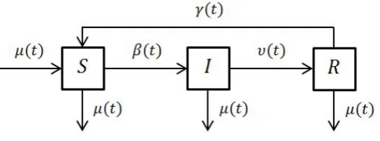
The aim of this section is constructing a mathematical model of a generalized epidemic SIRS (Susceptible, Infective, Recovered and Susceptible) model of the term
˙
S(t) =µ(t)−µ(t)S(t)−β(t)S(t)I(t) +γ(t)R(t), S(0) =S0 >0, (2.1) ˙
I(t) =β(t)S(t)I(t)−ν(t)I(t)−µ(t)I(t), I(0) =I0 >0, (2.2) ˙
R(t) =ν(t)I(t)−γ(t)R(t)−µ(t)R(t), R(0) =R0 >0, (2.3)
which is plotted in Figure 1 and modeling the spread of seasonal infectious disease under the following hypotheses:
1) The population is divided in three categories:
i. Susceptible S(t), who are all members are at risk becoming infected and individuals that have not the virus;
ii. Infected I(t), being all the infected individuals having the virus and able to transmit the illness;
iii. Recovered R(t), who are all the individuals not having the virus and with a temporary immunity.
Figure 1: Generalized SIRS model.
2) The birth and death rate µ(t)>0 being a continuous function. This means that ˙S(t) + ˙I(t) + ˙
3) The function β(t) between category S(t) and I(t), is a continuous T-periodic function, which is called transmission rate that satisfies:
0< βm = min
t∈[0,+∞]β(t)≤β(t)≤t∈max[0,+∞]β(t) = β M
and periodicity of the β(t), is to show the seasonality of the spread in the regional.
4) The rate of leaving the infective category I(t) is called ν(t) and similarity the rate of leaving the recoveredR(t) is γ(t) both of them are non-negative, continuous and bounded functions.
By setting R(t) = 1−S(t)−I(t) and using this expression in (2.1) and (2.2), we can obtain the following equivalent system:
˙
S(t) =k(t)−k(t)S(t)−β(t)S(t)I(t)−γ(t)I(t) (2.4) ˙
I(t) =β(t)S(t)I(t)−w(t)I(t), (2.5)
with S(0) =S0 >0 and I(0) =I0 >0 wherek(t) =µ(t) +γ(t) and w(t) =µ(t) +ν(t).
3. Dynamical properties of the solution
3.1. Positive solution of system (2.4)-(2.5)
In this subsection, we show that a solution of the system (2.4)-(2.5) with positive initial condition takes positive values.
Theorem 3.1. Let S(0) >0, and I(0) >0 and let (S(t), I(t))be a solution of system (2.4)-(2.5) on interval [0, t], then S(t)>0 and I(t)>0 for all t >0.
Proof . Let there is a pointt1 ∈(0, T) such thatt1 is the first point that satisfies S(t1) = I(t1) = 0. Firstly, we consider I(t1) = 0, and we know that I(t1) ≥ 0 for all t ∈ [0, t1] because I(0) > 0. We have
˙
I(t) = (β(t)S(t)−w(t))I(t)≥ min
0≤t≤t1{β(t)S(t)−w(t)}I(t).
Let m be defined as
m = min
0≤t≤t1{β(t)S(t)−w(t)}I(t),
where w(t) is defined in previous section. By (2.5) it follows that dI
dt ≥I(t)·m, for allt ∈[0, t1] and so,
I(t)≥kemt, for allt ∈[0, t1]
since I(0) =I0, therefork =I(0) and:
The above equation is true for 0≤t≤t0. This means thatI(t1)≥I(0)emt1 which is in contradiction with the assumption that I(t1) = 0.
Now, we suppose that S(t1) = 0 and note that I(t) ≥ 0 for 0 ≤ t ≤ t1, because I(0) > 0. By (2.4) at point t1 and the definition of k(t) andw(t) we obtain the following relation:
˙
S(t1) = k(t1)−k(t1)S(t1)−β(t1)S(t1)I(t1)−γ(t1)I(t1).
As S(t1) = 0 and alsok(t) = µ(t) +γ(t), thus the above expression is rewritten as following: ˙
S(t1) = µ(t1) +γ(t1)−γ(t1)I(t1)
=µ(t1) +γ(t1)(1−I(t1))≥µ(t1)>0,
because (1−I(t1))≥0. The above expression is a contradiction with the fact that for every 0≤t ≤T, we have S(0)>0 and S(t)>0, because implies that ˙S(t1)<0.
3.2. Globally asymptotically stable of a solution
Now, we consider the global stability of system (2.4)-(2.5). We start with the following definition [6, 14, 19, 20, 25].
Definition 3.2. X∗ = (S∗(t), I∗(t)) is a globally asymptotically stable solution of system (2.4)-(2.5), ifX∗ = (S∗(t), I∗(t))) is a bounded positive solution and for any other solutionX = (S(t), I(t)), the following relation for larget holds:
lim
t→+∞(|S(t)−S ∗
(t)|+|I(t)−I∗(t)|) = 0.
Theorem 3.3. If sgn(S(t)−z) = sgn(I(t)−z) for all z ∈ [mp, Mp], where mp > 0 and Mp > 0
such that mp ≤S(t), I(t)≤Mp, and also the hypothesis of the Chen theorem is held then the system
(2.4)-(2.5) has a unique positive stable T-periodic solution which is globally asymptotically.
Proof . Let (S∗(t), I∗(t)) be a positiveT-periodic solution of the system (2.4)-(2.5) and (S(t), I(t)) be any positive solution with initial conditions S(0)>0, I(0)>0. We define:
V(t) =|S(t)−S∗(t)|+|I(t)−I∗(t)|.
By calculating the upper right derivative ofV(t) along the solution of the system, it follows that:
DV(t) = sgn(S(t)−S∗(t))( ˙S(t)−S˙∗(t)) + sgn(I(t)−I∗
(t))( ˙I(t)−I˙∗(t))
with the definition of (S∗(t), I∗(t)) and (S(t), I(t)) we have:
DV(t) =sgn(S(t)−S∗(t))(−k(t)(S(t)−S∗(t))−β(t)(S(t)I(t)−S∗(t)I∗(t)) −γ(t)(I(t)−I∗(t)) + sgn(I(t)−I∗(t))(−w(t)(I(t)−I∗(t))
−β(t)(S(t)I(t)−S∗(t)I∗(t)).
If we suppose thatwm, wM, γm, γM, km and kM are real numbers defined by
wm = inf
0≤t≤+∞w(t), w
M = sup 0≤t≤+∞
w(t), γm = inf
0≤t≤+∞γ(t),
γM = sup
0≤t≤+∞
γ(t), km = inf
0≤t≤+∞k(t), k
M = sup 0≤t≤+∞
then
DV(t)≤ −Km|S(t)−S∗(t)| −sgn(S(t)−S∗(t))β(t)(S(t)I(t)−S∗(t)I∗(t)) −γmsgn(S(t)−S∗(t))(I(t)−I∗(t))−wm|I(t)−I∗(t)|
+ sgn(S(t)−S∗(t))β(t)(S(t)I(t)−S∗(t)I∗(t)),
and so
DV(t)≤ −Km|S(t)−S∗(t)| −γm(I(t)−I∗(t))−wm|I(t)−I∗(t)| ≤ −km|S(t)−S∗(t)| −(wm−γm)|I(t)−I∗(t)|
If we suppose thatα∗ = min{km, wm−γm} then we get
DV(t)≤ −α∗(|S(t)−S∗(t)|+|I(t)−I∗(t)|)
By integrating both sides of the above equation on the interval [0, t], it follows that:
Z t
0
DV(t)dt ≤ −α∗ Z t
0
(|S(t)−S∗(t)|+|I(t)−I∗(t)|)dt,
and so for all t≥0,
V(t)−V(0) ≤ −α∗ Z t
0
|S(t)−S∗(t)|dt−α∗ Z t
0
|I(t)−I∗(t)|dt,
and
V(t) +α∗ Z t
0
|S(t)−S∗(t)|dt+α∗ Z t
0
|I(t)−I∗(t)|dt
≤V(0) =|S(0)−S∗(0)|+|I(0)−I∗(0) <+∞.
By the above equation we conclude that, V(t) is bounded on[0, t] and also:
Z +∞
0
|S(t)−S∗(t)|dt <+∞, and
Z +∞
0
|I(t)−I∗(t)|dt <+∞.
Thus|S(t)−S∗(t)| ∈L1[0,+∞] and|I(t)−I∗(t)| ∈L1[0,+∞], on the other hand, since (S∗(t), I∗(t)) and (S(t), I(t)) are bounded for [T,+∞] and from the system (2.4)-(2.5) their derivatives are also bounded, then|S(t)−S∗(t)|and |I(t)−I∗(t)|are uniformly continuous on [T,+∞]. By the following lemma in [5] we have limt→+∞|S(t)−S∗(t)|= 0, limt→+∞|I(t)−I∗(t)|= 0.
4. Numerical results and discussion
The aim of this section is to apply the Runge-Kutta fourth order method (RK4 ) to solve systems of nonautonomous nonlinear differential equations (2.1)-(2.3) that describe the SIRS epidemic model. Runge-Kutta fourth order method is a numerical technique used to solve ordinary differential equation of the form [17]:
wheret0 = 0< t < T. Let h be the step time define by h= NT whereN is a positive integer number and the several nodesti given by ti =t0+ih, i= 0,1, . . . , N.
Analytical solution is defined by Y(t) and numerical solution is represented by Yi, where Yi is
approximation of Y(ti) where
Y=
S(t) I(t) R(t)
, Y0 =
S(0) I(0) R(0) ,
F(t,Y) =
f1(t, S, I, R)
f2(t, S, I, R)
f3(t, S, I, R)
=
µ(t)−µ(t)S(t)−β(t)S(t)I(t) +γ(t)R(t) β(t)S(t)I(t)−ν(t)I(t)−µ(t)I(t)
ν(t)I(t)−γ(t)R(t)−µ(t)R(t)
.
By using Fourth order Runge-Kutta method for the above system we have,
Yi+1 =Yi+
1
6[K1+ 2K2+ 2K3+K4], K1 =hF(ti,Yi),
K2 =hF(ti+
h 2,Yi+
1
2K1), K3 =hF(ti+
h 2,Yi+
1 2K2),
K4 =hF(ti+h,Yi+K3), i= 0,1, . . . , N.
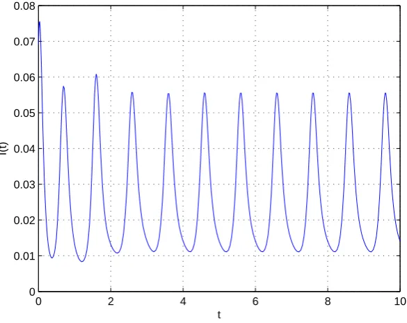
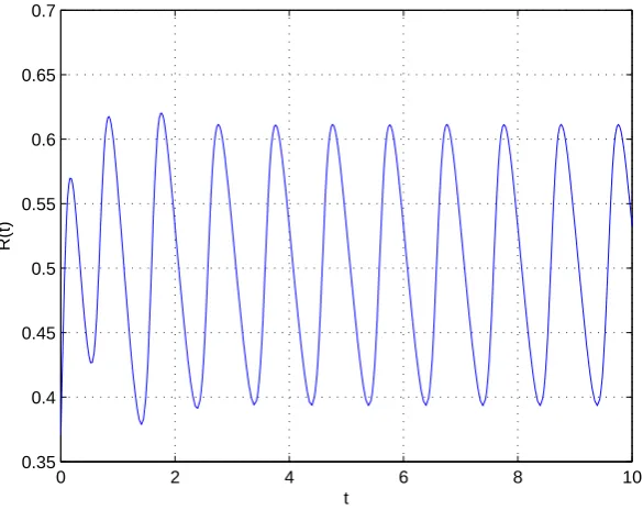
The numerical simulations were made using the parameter values showed in Table 4 and the RK4 algorithm is coded in the computer using Matlab package for obtaining numerical simulations. From Figures 2, 3 and 4 it can be seen that numerical results show that the Runge-Kutta method is accurate, easy to apply and the calculated solutions preserve the properties of the continuous models, such as the periodic behavior and positivity of solution.
Region b0 b1 ϕ µ θ γ
1 77 0.14 0.28 0.016 36 1.8
Table 1: Parameters values for system (2.1)-(2.3)
5. Conclusion
In this paper, we study the system of nonlinear of ordinary differential equations of the first order related to generalized epidemic model of infectious disease as a SIRS model. This model uses a trans-mission rate as a functionβ(t) periodic. Some qualitative properties of the solution are investigated. We show for positive initial conditions the solution of the equivalence system is positive and periodic. Moreover, under appropriate hypothesis the proposed model has a unique positive periodic solution which is globally asymptotically stable. Finally, the epidemic model is solved numerically using the RKM for approximating the solutions. Here, it is showed that the RKM is easy to apply and their numerical solutions preserve the properties of the models, such as positivity and periodic behavior.
References
0 2 4 6 8 10 0.35
0.4 0.45 0.5 0.55 0.6 0.65 0.7
t
s(t)
Figure 2: Approximate solutions ofS(t) by Runge-Kutta 4th order method andS0= 0.56.
0 2 4 6 8 10
0 0.01 0.02 0.03 0.04 0.05 0.06 0.07 0.08
t
I(t)
Figure 3: Approximate solutions ofI(t) by Runge-Kutta 4thorder method andI
0= 0.069.
[2] R.M. Anderson and R.M. May,Infectious Diseases of Humans: Dynamics and Control, Oxford University Press, 1991.
[3] D.F. Aranda, R.J. Villanueva, A.J. Arenas and G. Gonz´lez-Parra,Mathematical modeling of toxoplasmosis disease in varying size populations, Comput. Math. Appl. 56 (2008) 690–696.
[4] J. Arino,A multi-species epidemic model with spatial dynamics, Math. Med. Biol. 22 (2005) 129–142.
0 2 4 6 8 10 0.35
0.4 0.45 0.5 0.55 0.6 0.65 0.7
t
R(t)
Figure 4: Approximate solutions ofR(t) by Runge-Kutta 4th order method andR0= 0.371.
[6] F. Chen,Periodicity in a ratio-dependent predator-prey system with stage structure for predator,J. Appl. Math. 2 (2005) 153169.
[7] O. Diekmann and J.A.P. Heesterbeek,Mathematical Epidemiology of Infectious Diseases, Wiley, Chichester, 2000. [8] K. Dietz and D. Schenzle, (1985). Mathematical models for infectious disease statistics, In A celebration of
statistics, pp. 167–204. Springer, New York, NY, 1985.
[9] N.C. Grassly and C. Fraser, Seasonal infectious disease epidemiology, Proc. Royal Soc. B: Bio. Sci. 273 (2006) 2541–2550.
[10] D. Greenhalgh and I.A. Moneim,SIRS epidemic model and simulations using different types of seasonal contact rate,Syst. Anal. Model. Simul. 43 (2003) 573–600.
[11] W.H. vHamer,Epidemic disease in England,Lancet 1 (1906) 733–739.
[12] H.W. Hethcote, H.W. Stech and P. van den Driessche,Periodicity and stability in epidemic models: A survey,In Differential equations and applications in ecology, epidemics, and population problems, pp. 65–82. 1981.
[13] H.W. Hethcote,The mathematics of infectious diseases, SIAM Rev. 42 (2000) 599–653.
[14] Z. Jianga and J. Wei, (2008). Stability and bifurcation analysis in a delayed SIR model, Chaos, Solitons and Fractals 35 (2008) 609–619.
[15] L. Jodar, R.J. Villanueva and A.J. Arenas,Modeling the spread of seasonal epidemiological diseases: theory and applications,Math. Comput. Model. 48 (2008) 548–557.
[16] W.O. Kermack and A.G. McKendrick, Contributions to the Mathematical Theory of Epidemics, part 1, Proc. Roy. Soc. London Ser. A 115 (1927) 700–721.
[17] J.D. Lambert,Computational Methods in Ordinary Differential Equations,Wiley, New York, 1973.
[18] J. Ma and Z. Ma, Epidemics threshold conditions for seasonally forced SEIR models, Math. Biosci. Engin. 3 (2006) 161–172.
[19] Y. Muroya, Y. Enatsu and T. Kuniya, Global stability for a multi-group SIRS epidemic model with varying population sizes,Nonlinear Anal.: RWA 14 (2013) 1693–1704.
[20] S.M. O’Regan, T.C. Kelly, A. Korobeinikov and M.J.A. O’Callaghan, Lyapunov functions for SIR and SIRS epidemic models,Appl. Math. Lett. 23 (2010) 446–448.
[21] A.S. Perelson and P.W. Nelson,Mathematical analysis of HIV-I dynamics in vivo,SIAM Rev. 41 (1999) 3–44. [22] R. Ross,The Prevention of Malaria, 2nd ed,Murray, London, 1911.
[23] C.L. Seittos and L. Russos,Mathematical modeling of infectious disease dynamics,Virulence 4 (2013) 294–306. [24] Z. Shuai and V.D. Driessche, Global stability of infectious disease models using Lyapunov functions, SIAM J.
Appl. Math. 73 (2013) 1513–1532.
Solit. Fract. 44 (2011) 1106–1110.
[26] L. Wang and M.Y. Li, Mathematical analysis of the global dynamics of a model for HIV infection of CD4+T cells,Math. Biosci. 200 (2006) 44–57.
[27] A. Weber, M. Weber and P. Milligan, Modeling epidemics caused by respiratory syncytial virus (RSV), Math. Biosci. 172 (2001) 95–113.
[28] L. White, M. Waris, P. Cane, D. Nokes and G. Medley, The transmission dynamics of groups a and b human respiratory syncytial virus (hRSV ) in england and wales and finland: seasonality and cross-protection,Epidem. Infect. 133 (2005) 279–289.