Comments on the Adomian Decomposition Methods Applied to the KdV Equation

(1)

Published online November 20, 2013 (http://www.sciencepublishinggroup.com/j/acm) doi: 10.11648/j.acm.20130206.15

Comments on the Adomian Decomposition Methods

applied to the KdV equation

Mahmoud AKDI, Moulay Brahim SEDRA

Université Ibn Tofail, Faculté des Sciences, Département de Physique, LHESIR, Kénitra, Morocco

Email address:

[email protected](M. AKDI), [email protected] (M. B. SEDRA)

To cite this article:

Mahmoud AKDI, Moulay Brahim SEDRA. Comments on the Adomian Decomposition Methods Applied to the KdV Equation. Applied and Computational Mathematics. Vol. 2, No. 6, 2013, pp. 137-142. doi: 10.11648/j.acm.20130206.15

Abstract:

Based on previous works, especially [1] and [2], we try in the present contribution to study some new aspects of

the numerical solution of the KdV equation through the standard Adomian Decomposition Method.

The use of the multistage

Adomian Decomposition Method, applied to this equation, will be presented and discussed.

Keywords:

KdV Equation - Standard and Multistage Adomian Decomposition Methods

1. The Adomian Decomposition Method

(ADM)

Consider the KdV equation:

( )

3 3

6 0, ( , 0)

u

u x

f x

t

x

∂

₊

∂

₊

∂

₌

∂

which can be rewritten as follows:

( )

u

( ) ( )

x

f

x

N

Ru

t

u

₌

₋

₌

∂

0 ,

,

6 where

R

= ∂ ∂

3

/

x

3

represents the linear operator of the

KdV equation and

N u

( )

= ∂

u u

/

∂

x

is the non-linear

function. According to the ADM, the solution is expressed

by:

( )

,

( )

,

0

∑

∞ =

=

n

x

t

u

t

x

u

and the non-linear part:

( )

,

0

∑

∞ =

=

n n

A

u

N

with:

0 0

!

1

= ∞ =

























=

∑

λ

i i i n n

n

N

u

d

n

A

,

By integrating with respect to time and using the initial

conditions we have:

( )

0

( , )

( )

6. .

t

u x t

=

f x

−

∫



_

Lu

+

N u



_

ds

So,

( )

0 0

0

( , )

( )

,

6. .

t

n n

u x t

f x

L

u

x s

A

ds

∞ ∞ = =









=

−







+









∑



∫

For the KdV equation, the Adomian polynomials can be

expressed as follows:

∑

= −

∂

=

n i i n i n

x

u

A

0

This allows us to deduce

u

_n

( )

x t

,

namely

( )

[

]

0 1 0

,

0

t

n n n

u

x t

f x

u

₊

x t

Ru

A ds

n

=







= −

+

≥





∫

(2)

( )













=

2 sech

2

1

0 ,

2

x

u

We proceed in the following to compute

A

_n

( )

x t

,

and

( )

,

n

u

x t

for

n

∈

[ ]

0, 2

and try to determine the

approximate solution

U

ɶ

_n

( )

x t

,

using the following

formula:

( )

0

0 0

0

( , )

,

( )

,

6. .

n

n i

i

t n n

i i

U x t

f x

L

u x s

A ds

=

= =

=









=

−







+











∑

∫

ɶ

2. Study of the Discrepancy of the ADM

Applied to the KdV Equation

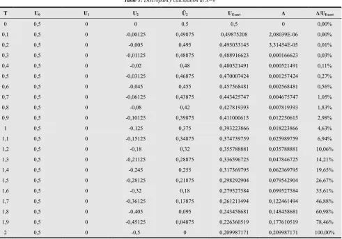
2.1. Calculation of Discrepancy

We present in this section some calculations by making

comparison between the values of approximated function

and the exact solution through space and time evolution. We

also evaluate the percentage of the discrepancy over the

exact solution.

Table 1: Discrepancy calculation at X=0

T U0 U1 U2 Ũ2 UExact ∆ ∆/UExact

0 0,5 0 0 0,5 0,5 0 0,00%

0,1 0,5 0 -0,00125 0,49875 0,49875208 2,08039E-06 0,00%

0,2 0,5 0 -0,005 0,495 0,495033145 3,31454E-05 0,01%

0,3 0,5 0 -0,01125 0,48875 0,488916623 0,000166623 0,03%

0,4 0,5 0 -0,02 0,48 0,480521491 0,000521491 0,11%

0,5 0,5 0 -0,03125 0,46875 0,470007424 0,001257424 0,27%

0,6 0,5 0 -0,045 0,455 0,457568481 0,002568481 0,56%

0,7 0,5 0 -0,06125 0,43875 0,443425747 0,004675747 1,05%

0,8 0,5 0 -0,08 0,42 0,427819393 0,007819393 1,83%

0,9 0,5 0 -0,10125 0,39875 0,411000615 0,012250615 2,98%

1 0,5 0 -0,125 0,375 0,393223866 0,018223866 4,63%

1,1 0,5 0 -0,15125 0,34875 0,374739759 0,025989759 6,94%

1,2 0,5 0 -0,18 0,32 0,355788881 0,035788881 10,06%

1,3 0,5 0 -0,21125 0,28875 0,336596725 0,047846725 14,21%

1,4 0,5 0 -0,245 0,255 0,317369795 0,062369795 19,65%

1,5 0,5 0 -0,28125 0,21875 0,298292904 0,079542904 26,67%

1,6 0,5 0 -0,32 0,18 0,279527584 0,099527584 35,61%

1,7 0,5 0 -0,36125 0,13875 0,261211494 0,122461494 46,88%

1,8 0,5 0 -0,405 0,095 0,243458681 0,148458681 60,98%

1,9 0,5 0 -0,45125 0,04875 0,226360519 0,177610519 78,46%

2 0,5 0 -0,5 0 0,209987171 0,209987171 100,00%

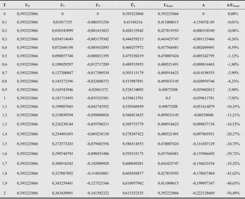
Table 2: Discrepancy calculation at X=0,5

0 0,470007424 0 0 0,470007424 0,470007424 0 0,00%

0,1 0,470007424 0,011511359 -0,000963568 0,480555216 0,480521491 -3,37243E-05 -0,01%

0,2 0,470007424 0,023022718 -0,00385427 0,489175872 0,488916623 -0,000259249 -0,05% 0,3 0,470007424 0,034534077 -0,008672108 0,495869393 0,495033145 -0,000836248 -0,17%

0,4 0,470007424 0,046045436 -0,015417081 0,500635779 0,49875208 -0,001883699 -0,38% 0,5 0,470007424 0,057556795 -0,024089189 0,50347503 0,5 -0,00347503 -0,70%

(3)

0,7 0,470007424 0,080579513 -0,047214811 0,503372127 0,495033145 -0,008338981 -1,68%

0,8 0,470007424 0,092090872 -0,061668324 0,500429972 0,488916623 -0,011513349 -2,35% 0,9 0,470007424 0,103602231 -0,078048973 0,495560683 0,480521491 -0,015039191 -3,13%

1 0,470007424 0,11511359 -0,096356756 0,488764258 0,470007424 -0,018756833 -3,99% 1,1 0,470007424 0,126624949 -0,116591675 0,480040698 0,457568481 -0,022472217 -4,91%

1,2 0,470007424 0,138136308 -0,138753729 0,469390003 0,443425747 -0,025964256 -5,86% 1,3 0,470007424 0,149647667 -0,162842918 0,456812173 0,427819393 -0,02899278 -6,78%

1,4 0,470007424 0,161159026 -0,188859242 0,442307208 0,411000615 -0,031306593 -7,62% 1,5 0,470007424 0,172670385 -0,216802702 0,425875107 0,393223866 -0,032651241 -8,30%

1,6 0,470007424 0,184181744 -0,246673296 0,407515872 0,374739759 -0,032776113 -8,75% 1,7 0,470007424 0,195693102 -0,278471026 0,387229501 0,355788881 -0,03144062 -8,84%

1,8 0,470007424 0,207204461 -0,31219589 0,365015995 0,336596725 -0,028419271 -8,44% 1,9 0,470007424 0,21871582 -0,34784789 0,340875355 0,317369795 -0,02350556 -7,41%

2 0,470007424 0,230227179 -0,385427025 0,314807579 0,298292904 -0,016514675 -5,54%

Table 3: Discrepancy calculation at X=1

0 0,393223866 0 0 0,393223866 0,393223866 0 0,00%

0,1 0,393223866 0,01817155 -0,000353256 0,41104216 0,411000615 -4,15455E-05 -0,01%

0,2 0,393223866 0,036343099 -0,001413023 0,428153942 0,427819393 -0,000334549 -0,08%

0,3 0,393223866 0,054514649 -0,003179302 0,444559213 0,443425747 -0,001133466 -0,26%

0,4 0,393223866 0,072686198 -0,005652093 0,460257972 0,457568481 -0,002689491 -0,59%

0,5 0,393223866 0,090857748 -0,008831395 0,475250219 0,470007424 -0,005242795 -1,12%

0,6 0,393223866 0,109029297 -0,012717209 0,489535955 0,480521491 -0,009014463 -1,88%

0,7 0,393223866 0,127200847 -0,017309534 0,503115179 0,488916623 -0,014198555 -2,90%

0,8 0,393223866 0,145372396 -0,022608372 0,515987891 0,495033145 -0,020954746 -4,23%

0,9 0,393223866 0,163543946 -0,02861372 0,528154092 0,49875208 -0,029402012 -5,90%

1 0,393223866 0,181715495 -0,035325581 0,539613781 0,5 -0,039613781 -7,92%

1,1 0,393223866 0,199887045 -0,042743952 0,550366959 0,49875208 -0,051614879 -10,35%

1,2 0,393223866 0,218058594 -0,050868836 0,560413625 0,495033145 -0,06538048 -13,21%

1,3 0,393223866 0,236230144 -0,059700231 0,569753779 0,488916623 -0,080837156 -16,53%

1,4 0,393223866 0,254401693 -0,069238138 0,578387422 0,480521491 -0,097865931 -20,37%

1,5 0,393223866 0,272573243 -0,079482556 0,586314553 0,470007424 -0,116307129 -24,75%

1,6 0,393223866 0,290744793 -0,090433486 0,593535173 0,457568481 -0,135966692 -29,72%

1,7 0,393223866 0,308916342 -0,102090928 0,600049281 0,443425747 -0,156623534 -35,32%

1,8 0,393223866 0,327087892 -0,114454881 0,605856877 0,427819393 -0,178037484 -41,62%

1,9 0,393223866 0,345259441 -0,127525346 0,610957962 0,411000615 -0,199957347 -48,65%

2 0,393223866 0,363430991 -0,141302322 0,615352535 0,393223866 -0,222128669 -56,49%

As we can easily observe, the convergence is limited

relatively to the time parameter, and it’s shown that it

diverge consistently beyond the value of τ

0

[1] defining the

(4)

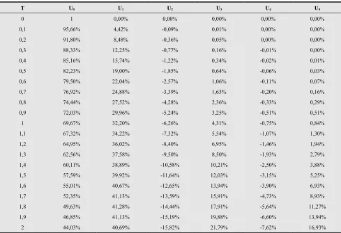
2.2. Determination of the Contribution of Each Element of

the Adomian Polynomial

In order to obtain a behavior of the evolving manner of the

elements of the Adomian polynomial, we elaborate the

calculation for

x

=

1 , to precise the percentage of each one

separately, as exposed in the following table:

Table 4: The evolving of Ui

T U0 U1 U2 U3 U4 U5

0 1 0,00% 0,00% 0,00% 0,00% 0,00%

0,1 95,66% 4,42% -0,09% 0,01% 0,00% 0,00%

0,2 91,80% 8,48% -0,36% 0,05% 0,00% 0,00%

0,3 88,33% 12,25% -0,77% 0,16% -0,01% 0,00%

0,4 85,16% 15,74% -1,22% 0,34% -0,02% 0,01%

0,5 82,23% 19,00% -1,85% 0,64% -0,06% 0,03%

0,6 79,50% 22,04% -2,57% 1,06% -0,11% 0,07%

0,7 76,92% 24,88% -3,39% 1,63% -0,20% 0,16%

0,8 74,44% 27,52% -4,28% 2,36% -0,33% 0,29%

0,9 72,03% 29,96% -5,24% 3,25% -0,51% 0,51%

1 69,67% 32,20% -6,26% 4,31% -0,75% 0,84%

1,1 67,32% 34,22% -7,32% 5,54% -1,07% 1,30%

1,2 64,95% 36,02% -8,40% 6,95% -1,46% 1,94%

1,3 62,56% 37,58% -9,50% 8,50% -1,93% 2,79%

1,4 60,11% 38,89% -10,58% 10,21% -2,50% 3,88%

1,5 57,59% 39,92% -11,64% 12,03% -3,15% 5,25%

1,6 55,01% 40,67% -12,65% 13,94% -3,90% 6,93%

1,7 52,35% 41,13% -13,59% 15,91% -4,73% 8,93%

1,8 49,63% 41,28% -14,44% 17,91% -5,64% 11,27%

1,9 46,85% 41,13% -15,19% 19,88% -6,60% 13,94%

2 44,03% 40,69% -15,82% 21,79% -7,62% 16,93%

2.3. Interpretation of the Results

As described in the previous table, the contribution of the

first elements of

U

i

, is more important at the beginning,

while we progress in the time calculation, and it gradually

decreases in favor of the other

U

i

elements. The

U

i

are

evolving in positive and negative values and progressively

their sum

Ũ

diverges from the exact solution.

So, the divergence cannot be attributed to special

categories of

U

i

, which we can avoid by implementing a

filter, but it is a mass fact. From where the interest to develop

other technique, that allow us to overcome the limitations of

the standard ADM.

3. Multistage Adomian Decomposition

Method (MS-ADM) for KdV

Equation

3.1. Principe of the Method

To simplify, we present the MS-ADM by the following

diagram:

     

=

2 sech . 2 1 )

(_x 2 x

f

n U~

( )i nxt U~ ,

) (

(5)

Based on this principle, we can write

( )

0

2

,

_t _0,1

f x

U

x t

=

ɶ

Hence, after calculation we found:

( )

(

)

(

)

2

4

1,79186.

0,819005

2,21. .

1

x x

x

e

f x

e

+

=

+

Using the previous backgrounds, we have to recalculate

the approximated function

*

( )

2

,

U

ɶ

x t

based on the new

expression of the initial condition

f

( )

x

, for:

t

=

t

₂

.

As made before for the standard Adomian decomposition

method and also taking into account the new formulation,

we have to precise the following expressions:

*

* * 0

0 0

U

A

U

x

∂

=

∂

;

* * *

1 0 0

0

t

U

= −

∫



_

RU

+

A



_

ds

;

* *

* * 1 * 0

1 0 1

U

A

U

x

∂

=

+

∂

;

* * *

2 1 1

0

t

U

= −

∫



_

RU

+

A



_

ds

.

3.2. Discrepancy Study

After calculation for

t

₂

=

0,15

, and in comparison with

the standard Adomian decomposition method, we present

the following results in the table below:

Table5: Discrepancies calculation

Values of X

0 0,25 0,5 0,75 1

Exact Solution 0,4971980 0,4987521 0,4849948 0,4575685 0,4195456

ADM 0,4971875 0,4988099 0,4851064 0,4577083 0,4196864

∆/ADM 0,0000105 -0,0000578 -0,0001116 -0,0001399 -0,0001407

MS-ADM 0,4881485 0,4734446 0,4525302 0,4256124 0,3918466

∆/MS-ADM 0,0090495 0,0253075 0,0324646 0,0319561 0,0276990

For establishing a better evaluation of these results, we

will elaborate a graphical representation of these functions:

• f

1

: the exact solution;

• f

2

: approximate solution using the standard

Adomian decomposition method;

• f

3

: approximate solution using the Multistage

Adomian decomposition method.

Graph 1: Comparative graphical representations

And for further richest visualization, we plot also these

function:

/

ADM Exact ADM MS ADM Exact MS ADM

F

U

F

U

∆

∆ − −



₌

₋



=

−



ɶ

(6)

Where:

• F

_∆_/_ADM

: is represented by the green color ;

• F

_∆_/_{MS ADM}₋

: is represented by the red color.

3.3. Discussion

Based on the previous numerical results and plotting

graphical representations, we can deduce the following

results:

1 Asymptotically, the both approximated functions

converge to the exact solution for this time value;

2 The discrepancy graphic for

F

∆/MS ADM−

, show that

this function evolve between +0,032 and -0,002 and

have single null value at

x

=

2,88

and after that

conserve a negative value;

3 The discrepancy graphic for

F

∆/ADM

, show that this

function have two null values for

x

=

0,037

and

2,33

x

=

and minimum for

x

=

0,881

, which it

means that this function conserve after his second zero,

a positive value.

Therefore, the both approximated functions are reaching

the exact solution, but not by the same manner. The positive

evolution for the function

F

_∆_/_ADM

, lead for the next

estimation processes of calculation of the Adomian

decomposition method, to the amplification of the

approximation error, contributing to it divergence.

Contrariwise, the Multistage Adomian decomposition

method have a more important positive discrepancy at the

beginning (in comparison with the Adomian decomposition

method), but it becomes negative for the rest of the spatial

parameter, while remaining near of 0.

4. Conclusion

Through this work, we were able to evolve with precision

the nature and the progression of the discrepancy between

the exact solution of KdV equation and the approximated

one using the standard Adomian decomposition method.

We have also, applied the Multistage Adomian

decomposition method to the resolution of the KdV equation,

which it allows us to elaborate a non-divergent method with

an acceptable accuracy level. Hence, the amplification of the

approximation error, as it occurs for the standard Adomian

decomposition method, is avoided.

Acknowledgements

The authors would like to express their thanks to Pr. Saad

CHOUKRI (EMI) for useful conversations.

References

[1] M.Akdi, M. B. Sedra, "Numerical KDV equation by the Adomian decomposition method", American Journal of Modern Physics. (2013)

[2] M. Akdi, "Study of solitary waves: results of resolution by numerical methods of the Korteweg-de Vries equation and simulation of the fluid flow", Ph. D. Thesis. (2013)

[3] M. Inc, On numerical solution of partial differential equation by the decomposition method, Kragujevac J Math. (2004) [4] García-Olivares, A., "Analytic solution of partial differential

equations with Adomian's

decomposition", Kybernetes (Bingley, U.K.: Emerald) 32: 354-368. (2003)

[5] García-Olivares, A., "Analytical solution of nonlinear partial differential equations of physics", Kybernetes (Bingley, U.K.: Emerald) 32: 548-560. (2003)

[6] Liao, S.J., "Homotopy Analysis Method in Nonlinear Differential Equation", Berlin & Beijing: Springer & Higher Education Press. (2012)

[7] G. Adomian, "Solving Frontier Problems of Physics: The Decomposition Method", Kluwer, Dordrecht. (1994) [8] K. Abbaoui and Y. Cherruault, Convergence of adomian’s

method applied to differential equations, Comp Math Appl. (1994)

[9] K. Abbaoui and Y. Cherruault, Convergence of Adomian’s method applied to nonlinear equations, Math Computer Model. (1994)

[10] N. Himoun, K. Abbaoui, and Y. Cherruault, New results of convergence of Adomian’s method,Kybernetes. (1999) [11] J. Biazar, E. Babolian, A. Nouri, R. Islam, "An alternate

algorithm for computing Adomian decomposition method in special cases", Appl. Math. Comput. 138, 1–7. (2003) [12] J. Biazar, M. Tango, E. Babolian, R. Islam, "Solution of the

kinetic modeling of lactic acid fermentation using Adomian decomposition method", Appl. Math. Comput. 139, 249–258. (2003)

[13] Kolebaje O. T., Ojo O. L., Akinyemi P., Adenodi R. A., "On the application of the multistage laplace adomian decomposition method with pade approximation to the rabinovich-fabrikant system", Advances in Applied Science Research. (2013)