Vol.8 (2018) No. 3
ISSN: 2088-5334
Developing an Artificial Neural Network Algorithm for Generalized
Singular Value Decomposition-based Linear Discriminant Analysis
Rolysent K. Paredes
#1, Ariel M. Sison
*, Ruji P. Medina
#2#
Graduate Programs, Technological Institute of the Philippines, Quezon City, Philippines, 1109 E-mail: [email protected], [email protected]
* School of Computer Studies, Emilio Aguinaldo College, Manila, Philippines, 1000 E-mail: [email protected]
Abstract— Artificial Neural Networks (ANN) form a dynamic architecture for machine learning and have attained significant
capabilities in various fields. It is a combination of interrelated calculation elements and derives outputs for new inputs after being trained. This study introduced a new mechanism utilizing ANN which was trained using Bayesian Regularization Back Propagation (BRBP) to improve the computational cost problem of the existing algorithm of the Generalized Singular Value Decomposition-based Linear Discriminant Analysis (LDA/GSVD). The proposed approach can minimize the number of iterations and mathematical processes of the existing LDA/GSVD algorithm which suffers time complexity. Through simulation using BLE RSSI Dataset from UCI which has 105 classes and 13 dimensions with 1420 instances, it was found out that ANN improved the computational cost during the classification of the data up to 57.14% while maintaining its accuracy. This new technique is recommended when classifying big data, and for pattern analysis as well.
Keywords— artificial neural network; bayesian regularization back propagation; generalized singular value decomposition; ANN for
LDA/GSVD; linear discriminant analysis.
I. INTRODUCTION
Classification is one of data mining’s approaches in which it is used to forecast, assign or predict hidden occurrences to their predefined groups [1]. It is mostly employed to evaluate a given dataset, consider each item of it, and allocates this item to a specific group [2]. There are some types of classification algorithms which include ID3, K-Nearest Neighbor (KNN) classifier, C4.5, Naive Bayes, Artificial Neural Network (ANN), Support Vector Machine (SVM), and Linear Discriminant Analysis (LDA) [2, 3].
Thus, it was found out that LDA outperformed other classification models and algorithms [3], and has been utilized widely in the previous years for dimensionality reduction, detection, and supervised learning [4]. It has been extensively employed as well in numerous applications [5-12]. It is supervised learning [13, 14] which intends for ideal conversion directions by reducing usual within-class scatter and make most of the average between-class scatter. Further, LDA has other advantages such as (a) inexpensive application; (b) adapts in discriminating non-linear datasets; and (c) coherence to Bayesian classification [15, 16]. Also, it surpasses PCA concerning classification performance [17].
It has the benefit of looking for projection vector that produces ideal discrimination among different collections of observations [18]. However, it fails when the matrix is singular due to small sample size (SSS) problem [8, 19, 20] which happens if the quantity of the training vectors is less than the dimensions. Because of that, the calculation of eigenvalues and eigenvectors becomes unbearable [4, 8, 20, 21].
widely used technique in solving SSS problem is the Generalized Singular Value Decomposition (GSVD) since it can overcome the mathematical problems integral in establishing the scatter matrices [28]. GSVD is also generally applied by various discriminant analysis approaches [21, 29], and a typical method for computing the matrix singular problems in different mathematical solutions [21, 30]. Moreover, GSVD on LDA (LDA/GSVD) provides extraordinary recognition accuracy [31] that is why many researchers used and developed variance of it. However, GSVD suffers from computational cost [12, 31-33] which can cause a longer time in classifying datasets when applied to LDA.
Thus, the purpose of the study is to improve the computational cost of LDA/GSVD by utilizing Artificial Neural Network (ANN). This technique will eliminate the mathematical computations and numerous iterations that are involved in the existing LDA/GSVD algorithm which compromise time complexity making it less efficient. Further, if there is a new instance for classification in the existing LDA/GSVD, the whole process of the algorithm will be repeated from the very start. With the proposed enhanced LDA/GSVD, learning can be done from the datasets and classify each instance, whether new or previously part of the training or testing, will be faster because it will not go back to the start of the whole procedure.
The use of ANN in developing the algorithm has the benefit of accuracy. Also, ANN is equipped with the uniqueness of concurrent processing, can learn and recall data relationships, and mapping of non-linear instances [34, 35]. It is also used in several mathematical calculations [36]. ANNs are applied in several real-world purposes because of their capability concerning resiliency and stableness even in noisy data and for its fault tolerance [37]. Thus, the widely employed method is Back Propagation Neural Network (BPNN). It is composed of input layer, hidden layers, and output layer [38]. An example of BPNN is Bayesian Regularization Back Propagation (BRBP). BRBP offers robust approximation for difficult and noisy inputs. Thus, it works excellently by removing network weights which have no impact on the problem solving and presents improvements on evading the problems of local minima [37]. Furthermore, it delivers weights into a training function while advancing the simplification performance of the old BPNN automatically [38].
Besides, the proposed new approach in this study aims to maintain the existing LDA/GSVD’s performance concerning its accuracy and to make its classification and prediction faster. Moreover, this new technique can also be adapted to other mathematical models or computations that implement GSVD.
A simulation of the existing LDA/GSVD algorithm has been presented for comparison with the results of the simulation having the new approach which is the utilization of ANN regarding the computational cost or time complexity, and accuracy.
II. MATERIAL AND METHOD
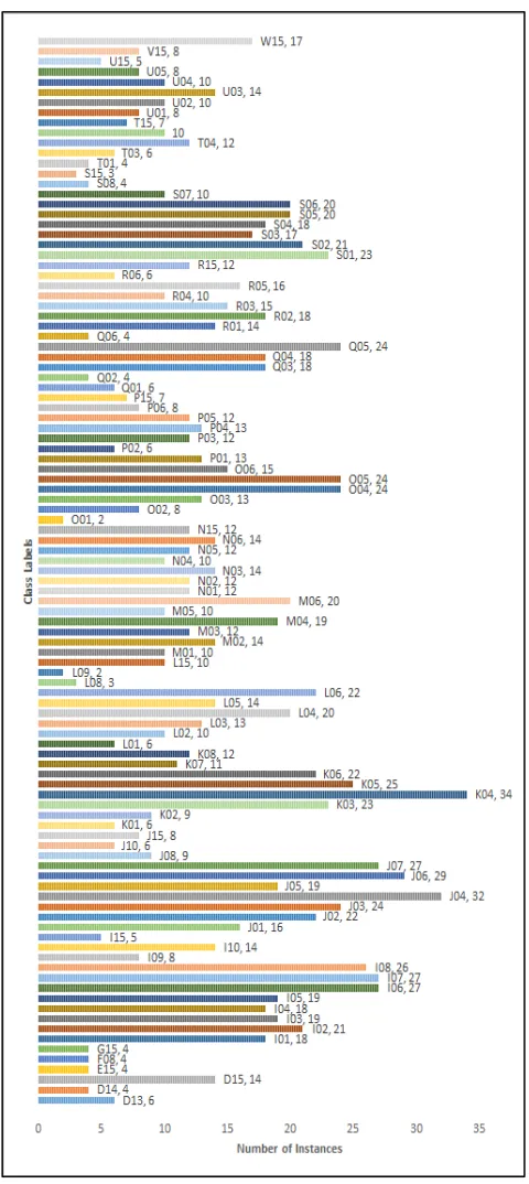
The study simulates the existing and the enhanced approach for LDA/GSVD algorithms. Dataset from UCI was used during the simulation. This dataset comprises RSSI readings collected from a collection of Bluetooth Low Energy (BLE) iBeacons in a practical indoor setting for navigation and localization applications. There are 105 classes, and 13 dimensions with 1420 instances in the dataset [39].
Table 1 shows parts of the dataset where dimensions are labeled initially from B3001 to B3013 which match to the 13 iBeacons. RSSI values are negative. Thus, more essential RSSI values designate closer adjacency to a certain iBeacon. A value of -200 implies that the iBeacon is very far. For class labeling, the column and row of the iBeacon’s position on the map are employed (e.g., I04 means that it is for column I, row 4).
TABLEI
PARTS OF BLERSSIDATASET
Class Label Dimension Name RSSI Value
I04
B3001 -75
B3002 -198
B3003 -200
B3004 -200
B3005 -200
B3006 -200
B3007 -200
B3008 -200
B3009 -74
B3010 -200
B3011 -200
B3012 -200
B3013 -200
O02
B3001 -200
B3002 -200
B3003 -200
B3004 -200
B3005 -200
B3006 -200
B3007 -200
B3008 -200
B3009 -74
B3010 -200
B3011 -200
B3012 -200
B3013 -200
U01
B3001 -200
B3002 -200
B3003 -200
B3004 -80
B3005 -200
B3006 -200
B3007 -200
B3008 -200
B3009 -200
B3010 -200
B3011 -200
B3012 -200
B3013 -200
F08, G15 and few others. Thus, it can lead to SSS problem on the classical LDA that is why LDA/GSVD shall be used.
Fig. 1 Classes and number of instances of the BLE RSSI dataset
The study introduced a new approach for LDA/GSVD by utilizing ANN. The tansigmoid transmission function was utilized for the hidden layers’ activation function. The flow of the procedure in training the enhanced algorithm is shown in figure 2, and the trained network’s architecture is presented in figure 3. The ANN architecture is formed from 13 input variables which are the dimensions, and the corresponding 13 output variables are the expected feature subspaces. For the architecture to learn and predict the
possible outcomes, the feature subspaces must be derived from the existing LDA/GSVD algorithm (table 2) since each dimension will have a corresponding feature subspace.
These dimensions and feature subspaces will be used in training and testing. For the sampling, 70% of the instances of the dataset were allocated for training, and 30% for the testing. Moreover, in training of the network, Bayesian Regularization Back Propagation (BRBP) was employed.
TABLEII
EXISTINGLDA/GSVDALGORITHM
Algorithm: Existing LDA/GSVD Algorithm
For the matrix A ∈ Rm×n with k groups, it calculates the matrix’s columns G ∈ Rm×(k−1), which maintains the configured cluster
dimensionally narrowed space, and determines (k − 1)-dimensional depiction Y of A.
Step 1: Calculate Hw ∈ Rm×n and Hb ∈ Rm×k from A
Step 2: Solve the K = (Hb,Hw)T ∈ R(k+n)×m for its orthogonal decomposition.
Step 3: Let t = rank(K).
Step 4: Calculate W from the SVD of P(1 : k,1 : t), which is
UTP(1 : k,1 : t) W = ΣA.
Step 5: Solve the first k − 1 columns of
and allocate those to G. Step 6: Y = GTA.
After saving the trained network, it will become a module or subroutine that will be used to solve the expected new feature subspaces of the inputs. Thus, the algorithm (table 3) was used to compute the feature subspaces of the instances of the BLE RSSI dataset.
Fig. 3 Artificial Neural Network Architecture for the LDA/GSVD algorithm
TABLEIII
COMPUTATION OF THE FEATURE SUBSPACES USING THE ENHANCED
LDA/GSVD ALGORITHM
Algorithm: Computation of the Feature Subspaces 1. Enter the 13 values of the 13 dimensions.
2. Compute the 13 feature subspaces using the module from the trained network.
3. Return the computed feature subspaces.
III.RESULT AND DISCUSSION
Using MATLAB R2014a, both algorithms, existing and enhanced LDA/GSVD, were coded and ran on a PC with the processor of Intel® Core i5, 4GB RAM, and 2.7GHz speed.
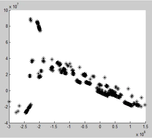
A. Dataset without LDA/GSVD Classification
Figure 4 below shows the graphical representation of the data without performing LDA/GSVD. Since the dataset is multi-dimensional, for this example, only the first two dimensions are shown in the graph. It can be seen that instead of 105 classes, data points are grouped in approximately three (3) classes. Thus, all of these data points cannot be distinguished as to what classes they belong.
Fig. 4 Graph of the dataset without applying LDA/GSVD
B. Existing LDA/GSVD Algorithm
For classifying 105 classes with 13 dimensions, and a total of 1420 instances, the LDA/GSVD algorithm took 7 seconds to finish. The computational cost was obtained using equation 1.
CC = ET – ST (1)
Where CC is the computational cost, ET means end time or the time when the program finished to execute all the instructions), and ST means start time or the time when the program starts to execute.
Figure 5 shows the graph for the feature subspaces of the first two dimensions of the dataset using the existing LDA/GSVD. Also, figure 5 shows a better separation of data points compared to figure 4. Due to the number classes and instances, most of the data points with same feature subspaces overlap with each other.
Fig. 5 Graph of the feature subspaces after applying LDA/GSVD
C. Enhanced LDA/GSVD
The performance functions were used in the study which includes the Mean Squared Error (MSE) and Regression (R) to evaluate the performance of the ANN for LDA/GSVD algorithm. MSE is the average squared difference between experimental output values and the fed targets in training.
(2)
Where n is the sample set’s size, ai is the ANN
experimental or observed output and ti is the matching
targets. Regression (R) computes the outputs and targets’ correlation. When the value of R is 1, it signifies a good or close relationship, otherwise a random relationship [38].
Figure 6 depicts the performance of training and test samples using BRBP algorithm. The graph shows that the test and training samples overlap with each other. Thus, training and test curves continue to stabilize every time the epoch increments. At epoch 1500 the MSE error is approximately 2.5115 x10⁻³. Further, the histogram in figure 7 presents the frequency of the instances per error. The measurement of the error is by subtracting the targets and the
Hidden Layer: 30 hidden neurons Input
Layer:
1420 instances
by 13 dimensions
Output Layer: 13
resultant outputs. The most significant error in the training was at around 0.2443.
Fig. 6. BRBP’s Prediction Result
Fig. 7. BRBP’s Histogram of Error Sequences
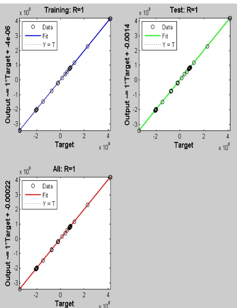
Figure 8 shows BRBP algorithm’s correlation. Thus, the graphs present that the algorithm is accurate and better because the MSE is less than zero and the value of R for the training, test, and overall analysis is 1. Further, table 4 shows the performance of the enhanced LDA/GSVD.
TABLEIV
PERFORMANCE OF ANN ALGORITHM FOR LDA/GSVD USING BRBP
Dataset Sample Mean Square Error Regression
Training 5.6896e-05 1
Testing 6.1412e-05 1
Fig. 8. BRBP’s Regression Analysis
Fig. 9 Graph of the feature subspaces after applying the enhanced LDA/GSVD
It is noticeable that figure 9 above which presents the graph of the feature subspaces using the enhanced algorithm is very much similar to figure 5 which utilized the existing LDA/GSVD. It is a manifestation that the accuracy of the improved LDA/GSVD maintains the accuracy of current LDA/GSVD algorithm.
because there are only 1420 instances that composed the dataset.
TABLEV
COMPUTATIONAL COSTS OF THE EXISTING AND ENHANCED ALGORITHMS
Algorithm STa ETb CCc
Existing
LDA/GSVD 08:51:02 08:51:09 7 seconds
Enhanced
LDA/GSVD 09:35:43 09:35:46 3 seconds
Improvement of the Enhanced LDA/GSVD 57.14%
a. Start Time, b. End Time, c. Computational Costs
IV.CONCLUSIONS
Simulation results showed that enhanced LDA/GSVD using ANN outperformed the existing LDA/GSVD algorithm regarding computational cost during the classification of the datasets. Thus, it makes the new approach an efficient way of doing LDA/GSVD. It is also evident in the simulation that the new technique using BRBP can obtain the best performance of accuracy by increasing the number of epochs. With that, the new mechanism is highly recommended especially if the dataset has many instances and dimensions due to its lower computational cost. Moreover, implementation of the enhanced LDA/GSVD algorithm to big data will be the next research to be done.
ACKNOWLEDGMENT
The authors would like to thank the Management Information Systems department of Misamis University, Ozamiz City, Philippines for the big help for the success of the study.
REFERENCES
[1] W. Hadi, F. Aburub, and S. Alhawari, “A new fast associative classification algorithm for detecting phishing websites,” Appl. Soft Comput., vol. 48, pp. 729–734, Nov. 2016.
[2] S. S. Nikam, “A comparative study of classification techniques in data mining algorithms,” Oriental Journal of Computer Science and Technology, vol. 8, no. 1, pp. 13-19, 2015.
[3] N. B. M. Zainee and K. Chellappan, “A preliminary dengue fever prediction model based on vital signs and blood profile,” 2016 IEEE EMBS Conference on Biomedical Engineering and Sciences (IECBES), pp. 652-656, 2016.
[4] P. P. Markopoulos, “Linear Discriminant Analysis with few training data,” 2017 IEEE International Conference on Acoustics, Speech and Signal Processing (ICASSP), pp. 4626-4630, March 2017.
[5] X. Gao, X. Wang, X. Li, and D. Tao, “Transfer latent variable model based on divergence analysis,” Pattern Recognition, vol. 44, no. 10-11, pp. 2358–2366, 2011.
[6] X. Gao, X. Wang, D. Tao, and X. Li, “Supervised Gaussian Process Latent Variable Model for Dimensionality Reduction,” IEEE Transactions on Systems, Man, and Cybernetics, Part B (Cybernetics), vol. 41, no. 2, pp. 425–434, 2011.
[7] J. J. D. M. S. Junior and A. R. Backes, “Shape classification using line segment statistics,” Information Sciences, vol. 305, pp. 349–356, 2015.
[8] J. Shao, Y. Wang, X. Deng, and S. Wang, “Sparse linear discriminant analysis by thresholding for high dimensional data,” The Annals of Statistics, vol. 39, no. 2, pp. 1241–1265, 2011.
[9] D. Tao, J. Cheng, X. Lin, and J. Yu, “Local structure preserving discriminative projections for RGB-D sensor-based scene classification,” Information Sciences, vol. 320, pp. 383–394, 2015. [10] D. Wang, X. Gao, and X. Wang, “Semi-Supervised Nonnegative
Matrix Factorization via Constraint Propagation,” IEEE Transactions on Cybernetics, vol. 46, no. 1, pp. 233–244, 2016.
[11] L. Zhang, L. Wang, and W. Lin, “Generalized Biased Discriminant Analysis for Content-Based Image Retrieval,” IEEE Transactions on
Systems, Man, and Cybernetics, Part B (Cybernetics), vol. 42, no. 1, pp. 282–290, 2012.
[12] H. Zhao and P. C. Yuen, “Incremental Linear Discriminant Analysis for Face Recognition,” IEEE Transactions on Systems, Man, and Cybernetics, Part B (Cybernetics), vol. 38, no. 1, pp. 210–221, 2008. [13] C. L. Liu, W. H. Hsaio, C. H. Lee, and F. S. Gou, “Semi-Supervised
Linear Discriminant Clustering,” IEEE Transactions on Cybernetics, vol. 44, no. 7, pp. 989–1000, 2014.
[14] J. Zhao, L. Shi, and J. Zhu, “Two-Stage Regularized Linear Discriminant Analysis for 2-D Data,” IEEE Transactions on Neural Networks and Learning Systems, vol. 26, no. 8, pp. 1669–1681, 2015. [15] G. Baudat and F. Anouar, “Generalized Discriminant Analysis Using
a Kernel Approach,” Neural Computation, vol. 12, no. 10, pp. 2385– 2404, 2000.
[16] S. Mika, G. Ratsch, J. Weston, B. Scholkopf, and K. Mullers, “Fisher discriminant analysis with kernels,” Neural Networks for Signal Processing IX: Proceedings of the 1999 IEEE Signal Processing Society Workshop, pp. 41-48, 1999.
[17] A. Sharma and K. K. Paliwal, “Linear discriminant analysis for the small sample size problem: an overview,” International Journal of Machine Learning and Cybernetics, vol. 6, no. 3, pp. 443–454, Jul. 2014.
[18] S. Yu, Z. Cao, and X. Jiang, “Robust linear discriminant analysis with a Laplacian assumption on projection distribution,” 2017 IEEE International Conference on Acoustics, Speech and Signal Processing (ICASSP), pp. 2567-2571, 2017.
[19] W. Deng, J. Hu, and J. Guo, “Extended SRC: Undersampled Face Recognition via Intraclass Variant Dictionary,” IEEE Transactions on Pattern Analysis and Machine Intelligence, vol. 34, no. 9, pp. 1864–1870, 2012.
[20] Z. Wang, Y.-H. Shao, L. Bai, C.-N. Li, L.-M. Liu, and N.-Y. Deng, “MBLDA: A novel multiple between-class linear discriminant analysis,” Information Sciences, vol. 369, pp. 199–220, 2016. [21] X. Jing, Y. Dong, and Y. Yao, “Uncorrelated optimal discriminant
vectors based on generalized singular value decomposition,” International Conference on Automatic Control and Artificial Intelligence (ACAI 2012), 2012.
[22] T. Zhang, B. Fang, Y. Y. Tang, Z. Shang, and B. Xu, “Generalized Discriminant Analysis: A Matrix Exponential Approach,” IEEE Transactions on Systems, Man, and Cybernetics, Part B (Cybernetics), vol. 40, no. 1, pp. 186–197, 2010.
[23] D. Cai, X. He, and J. Han, “Training Linear Discriminant Analysis in Linear Time,” 2008 IEEE 24th International Conference on Data Engineering, pp. 209-217, Apr. 2008.
[24] Z. Zhang, G. Dai, C. Xu, and M. I. Jordan, “Regularized discriminant analysis, ridge regression and beyond,” Journal of Machine Learning Research, pp. 2199-2228, Aug. 11, 2010.
[25] H. Yu and J. Yang, “A direct LDA algorithm for high-dimensional data — with application to face recognition,” Pattern Recognition, vol. 34, no. 10, pp. 2067–2070, 2001.
[26] J. Ye and Q. Li, “A two-stage linear discriminant analysis via QR-decomposition,” IEEE Transactions on Pattern Analysis and Machine Intelligence, vol. 27, no. 6, pp. 929–941, 2005.
[27] J. K. P. Seng and K. L.-M. Ang, “Big Feature Data Analytics: Split and Combine Linear Discriminant Analysis (SC-LDA) for Integration Towards Decision Making Analytics,” IEEE Access, vol. 5, pp. 14056–14065, 2017.
[28] P. Howland and H. Park, “Generalizing discriminant analysis using the generalized singular value decomposition,” IEEE Transactions on Pattern Analysis and Machine Intelligence, vol. 26, no. 8, pp. 995– 1006, 2004.
[29] C. H. Park and H. Park, “A Relationship between Linear Discriminant Analysis and the Generalized Minimum Squared Error Solution,” SIAM Journal on Matrix Analysis and Applications, vol. 27, no. 2, pp. 474–492, 2005.
[30] Z. Chen and T. H. Chan, “A truncated generalized singular value decomposition algorithm for moving force identification with ill-posed problems,” Journal of Sound and Vibration, vol. 401, pp. 297– 310, 2017.
[31] W. Wu and M. O. Ahmad, “Orthogonalized linear discriminant analysis based on modified generalized singular value decomposition,” 2009 IEEE International Symposium on Circuits and Systems, pp. 1629-1632, 2009.
[33] M. Berry, D. Mezher, B. Philippe, and A. Sameh, “Parallel computation of the singular value decomposition,” INRIA, 2003. [34] Y. Dash, and S. K. Dubey, “Quality prediction in object oriented
system by using ANN: a brief survey.” International Journal of Advanced Research in Computer Science and Software Engineering, vol. 2, no. 2, 2012.
[35] S. S. Ranhotra, A. Kumar, M. Magarini, and A. Mishra, “Performance comparison of blind and non-blind channel equalizers using artificial neural networks,” 2017 Ninth International Conference on Ubiquitous and Future Networks (ICUFN), pp. 243-248, July 2017.
[36] H. Tana, G. Yang, B. Yu, X. Liang, and Y. Tang, “Neural Network Based Algorithm for Generalized Eigenvalue Problem,” 2013 International Conference on Information Science and Cloud Computing Companion, pp. 446-451, 2013.
[37] K. Jazayeri, M. Jazayeri, and S. Uysal, “Comparative Analysis of Levenberg-Marquardt and Bayesian Regularization Backpropagation Algorithms in Photovoltaic Power Estimation Using Artificial Neural Network,” Advances in Data Mining. Applications and Theoretical Aspects Lecture Notes in Computer Science, pp. 80–95, July 2016. [38] F. Dalipi and S. Y. Yayilgan, “The impact of environmental factors
to skiing injuries: Bayesian regularization neural network model for predicting skiing injuries,” 2015 6th International Conference on Computing, Communication and Networking Technologies (ICCCNT), pp. 1-6, July 2015.