Analytical Available Bandwidth Estimation in Wireless Ad-hoc Networks Considering Mobility in 3-Dimensional Space

Scalable Computing: Practice and Experience

Volume 20, Number 2, pp. 317–333. http://www.scpe.org

ISSN 1895-1767 c

⃝2019 SCPE

ANALYTICAL AVAILABLE BANDWIDTH ESTIMATION IN WIRELESS AD-HOC NETWORKS CONSIDERING MOBILITY IN 3-DIMENSIONAL SPACE

MUKTA∗_{AND NEERAJ GUPTA}†

Abstract. Estimation of available bandwidth for ad hoc networks has always been open and active challenge for the researchers. A lot of literature is proposed in the last 20 years to evaluate the residual bandwidth. The main objective of the work being admission of new flow in the network with the constraint that any existing current transmission is not affected. One of the prime factors affecting the estimation process is the collision among packets. These collisions trigger the backoff algorithm that leads to wastage of the usable bandwidth. Although a lot of state of art solutions were proposed, but they suffer from various flaws and shortcoming. Other factor contributing to the inaccuracy in existing solution is the mobility of nodes. Node mobility leads to instability of links leading to data losses and delay which impact the bandwidth. The current paper proposes an analytical approach named Analytical Available Bandwidth Estimation Including Mobility (AABWM) to estimate ABW on a link. The major contributions of the proposed work are: i) it uses mathematical models based on renewal theory to calculate the collision probability of data packets which makes the process simple and accurate, ii) consideration of mobility under 3-D space to predict the link failure and provides an accurate admission control. Extensive simulations in NS-2 are carried out to compare the performance of the proposed model against the existing solutions.

Key words: QoS, available bandwidth, analytical, collision, mobility, fixed point analysis, 3 dimensions

AMS subject classifications. 68M10, 68M20, 60K05, 60K25

1. Introduction. Recently, the development of multimedia applications like live movies, video on demand, e-learning etc. has necessitated the provision of QoS in MANETs. All these applications have diversified requirement in terms of QoS parameters. Some are sensitive to delay while others may demand guaranteed bandwidth for the smooth flow in the network. Thus, an accurate prediction of the available resources is required for the QoS flow guarantee. Bandwidth is one of the scarce resources and should be distributed wisely among the different flows such that admission of new flows doesn’t deteriorate the performance of existing flows. Therefore, an accurate estimation of its availability is much required for the true admission control. Imprecise estimation of the ABW leads to false admission control whose bandwidth consumption is more than the estimated ABW. Some approaches like BRuIT [1], CACP [2], AAC [3] didn’t address the impact of collisions while estimating the ABW thus provide false admission control, whereas ABE [4] addressed this issue but may results erroneous estimation. It was observed that estimation errors are mainly due to two reasons: first is the bad computation of the considered network criteria such as collision and integrating the same in the estimation; the second is failure to capture each of the network criteria affecting the bandwidth.

ABE [4] focused on few main challenges to evaluate the ABW on a link: idle period synchronization, collision probability and average backoff period between two transmissions. Authors in [4] utilizes the rate of exchange of HELLO packets to compute the collision probability. To handle the discrepancy that arises due to the smaller size of HELLO packets, the resultant is interpolated using Lagrange interpolating polynomial to get the collision rate of data packets. This leads to followings limitations: i) polynomial is calculated at a node for a specific scenario and same is applicable for all nodes or for any scenarios, ii) experiment needs to be executed in advance to calculate the collision probability, iii) HELLO packets that are sent late or lost due to network congestion or overloaded medium are combined with the computed collision rate which overestimates its impact. To remove all these limitations, we proposed to use an analytical approach using fixed point analysis based on renewal theory for the computation of collision probability under heterogeneous network conditions. Most of the available literature assumed homogeneous condition to simplify the process involved. But real time network conditions are heterogeneous in nature consisting of nodes having different capabilities and resources such as transmission rate, battery life, radio range, etc. The major benefits of our proposed solution include: predict the result set when the network parameters get varied, simple and easy approach to compute the collisions without using Hello packets.

∗_{Computer Science Department, K. R. Mangalam University, Gurgaon, India, ([email protected]).} †_{Computer Science Department, K. R. Mangalam University, Gurgaon, India, ([email protected]).}

Another cause of error is neglecting the important criteria such as mobility which is not addressed in many of the available literature. Mobility of nodes causes the frequent link breakage and re-construction of links leading to delay and loss of data packets. To overcome the above issue, the current paper considered the bandwidth loss due to mobility of nodes under 3-dimensional space and observed its effects on admission control. Results obtained using our proposed solution is compared with existing solutions which show the improvement done by our proposed approach.

The paper is organized as follows: Section 2 gives an insight into existing available bandwidth estimation techniques and admission control solutions. Section 3 presents our proposed approach AABWM for the esti-mation of ABW considering all the network criteria affecting the bandwidth under heterogeneous conditions. Section 4 introduces the mobility model under 3-dimensional space to predict the link persistent factor for the improvement in ABW estimation and thus the admission control. Section 5 presents the comparative analysis of results obtained using our proposed solution with the existing approaches under two cases: stationary nodes and mobile nodes. Finally, Section 6 concludes the paper.

2. Related work. The bandwidth estimation techniques can be classified into three main categories: Active techniques, Passive techniques and Analytical techniques. Active techniques emit probe packets at multiple rates between sender and receiver node. By measuring the packets inter-arrival time at the receiver node estimates the end-to-end ABW along a path. The emission rate of these probe packets is increased gradually by the sender node until the congestion arises in the network. SLoPS [5] and TOPP [6] approaches come under this category. Active techniques burden the network with probe packets which can lead to network congestion and consuming precious network resources. Loss of probe packets due to network congestion or overloaded medium may provide the erroneous measurement. These drawbacks make such techniques inefficient to be employed in mobile ad hoc networks. To avoid these drawbacks, the passive techniques monitor the radio channel activities including transmission, reception or idle periods of channel in its vicinity over a certain period of time. The available bandwidth is determined by evaluating the channel usage ratio of nodes in the network. These techniques are non-intrusive in nature. Some major solutions that falls in this category includes: BRuIT [1], CACP [2], AAC [3]. Most of these techniques failed to address the problem associated due to collisions among the packets. The packet collisions consumes the network resources and adversely affect the ongoing transmission in the network.

Authors in [4] addressed these challenges and proposed a solution by incorporating the impact of collisions and time period consumed due to backoff on the bandwidth estimation. To calculate the collision probability [4] utilizes the HELLO packets. By counting the total number of received HELLO packets in a given interval of time and comparing this number with the actual number of received HELLO packets provides the collision probability of HELLO packets. The authors interpolate the resultant using Lagrange interpolating polynomial to compute the collision probability for the data packets of varying size. This approach suffers from the limitations as mentioned in Sec. 1 which makes this technique inefficient for ABW estimation. IAB [7] is a similar approach as that of [4] except that it differentiates the channel busy state due to packet transmission or reception from that of carrier sensing mechanism. Authors in [8] proposed a solution DLI-ABE for bandwidth estimation by employing the Distributed Lagrange interpolating polynomial which is to be calculated separately for each node in any scenario before transmitting the data. All the above-mentioned approaches rely on frequent exchange of Hello packets for calculating the collision probability which contradicts the non-intrusive nature of the passive technique. Moreover, the above literature assumes that the position of the node is static, i.e. there is no mobility. No satisfactory solution is obtained from any of above techniques to estimate the collision probability and their effect on backoff. Analytical techniques provide the reliable solution for the above problem. These techniques are having advantage of predicting the result set by varying the network parameters. Different analytical models available in the literature are based on: i) Bi-dimensional Markov chain, ii.) Means value argument, iii) fixed point analysis based on renewal theory. Based on the traffic conditions, these networks are further divided into two sub-categories: saturated and non-saturated networks. In saturated conditions node always has next packet available to transmit after completing the current transmission; whereas, in non-saturated condition node’s buffer may be empty some time.

Fig. 3.1.Total overlap of idle time periods.

based on the Markov chain were extended to incorporate various challenges like error-prone channel, non-saturated environment, heterogeneous traffic conditions and many other. The major work in literature can be referred in [10, 11, 12, 13, 14, 15]. The solution based on Markov chain are complex and mathematical expressions are computationally extensive. Authors in [16] presented a simple approach using fixed point analysis based on renewal theory. The results obtained are synchronous with the result of [9]. Authors in [17] extended the approach of [16] for non-saturated network condition. Most of analytical models didn’t addresses the problem associated with mobility of nodes. The authors in [18] presented a novel approach named Improved Bandwidth Estimation through Mobility incorporation (IBEM) for the estimation of ABW on a link by incorporating the mobility criteria during bandwidth estimation. The authors in [18] ignore the effects of elevation and height while predicting the link failure due to mobility of nodes. Authors in [19] calculate the collision probability based on Markov chain under the assumption of saturated condition.

3. AABWM approach for ABW estimation. The main contribution of this paper is to determine the available bandwidth in mobile ad hoc networks using the analytical models based on renewal theory. To address the various challenges for predicting ABW in mobile ad hoc networks the work is divided into four sections: i) idle period synchronization ii) impact of collision probability iii) effect of average backoff period iv) mobility issues.

3.1. Synchronization of idle time periods between sender and receiver node. For efficient com-munication to happen, the information about the bandwidth consumption at each node and its neighborhood is much necessitated. The ABW at a node is evaluated by monitoring the radio channel activities of the node in its vicinity. A node is considered as busy when it is either transmitting or receiving information on the channel. Thus, the ABW at a node is evaluated by measuring the idle and busy period of nodes in the network. The upper bound for estimating ABW can be expressed as [20]:

ABWi= ti

T.Cmax

(3.1)

where, ti represents the idle periods sensed by node iduring the total measurement duration T and Cmax is the raw channel capacity.

Lettsandtrrepresents the idle periods of sendersand receiverrrespectively, evaluated using (3.1) during the measurement period T. Fig. 3.1 and Fig. 3.2 depicts the two extreme cases (full overlap and no overlap) of node’s overlap period respectively to evaluate the ABW on a link.

Fig. 3.1 represents the case where idle period of both sender node and receiver node completely overlap to each other. In other words, the channel is idle at both the ends make transmission of packet a successful event. Thus, the communication is feasible only when the idle periods of sender (ts) and receiver (tr) overlap each other for the period of the transmission as stated in [3]. This type of communication is possible using a precise clock synchronization mechanism. Thus, the ABW on a link constituting between sender s and receiver r is given by [3] as:

ABWlink(s,r)= min( ts T,

tr T)

(3.2)

Fig. 3.2.No overlap of idle time periods.

and the available bandwidth on a link is counted as null. It can be concluded that the ABW on a link is dependent on the overlap period of idle time at both sender node and the receiver node for successful communication to happen.

Authors in [4] propose to incorporate a probabilistic approach and used the average of the idle time periods of sender and receiver to evaluate the ABW on a link. Thus, the ABW on a link is given as:

ABWABE(s,r)= ts T.

tr T.Cmax

(3.3)

Where ts and tr represent the idle periods of sender(s) and receiver(r) respectively, during the measurement period T; Cmaxis the maximum channel capacity.

3.2. Collision Probability using Fixed point analysis (FPA). The ABW calculated using (3.3) provides a conservative solution for estimation of ABW. Collision impacts the bandwidth estimation process adversely. Collisions can occur due to various reasons including Hidden terminal problem and Exposed terminal problem. A packet transmitted by a node may collide with the other packet transmitted by other nodes in its vicinity leading to delay and wastage of bandwidth. Thus, it is imperative to accurately predict the collisions in the network otherwise the estimation becomes fallacious. The authors in [4] addressed this issue and presented a mathematical framework for the estimation of ABW on a link on account of the collision. Mathematically the same can be represented as:

ABWABE(s,r)= ts T.

tr

T.Cmax.(1−p).(1−k)

(3.4)

Where p represents the collision probability of data packets, and k represent the proportion of bandwidth consumed due to backoff mechanism in the event of the collision.

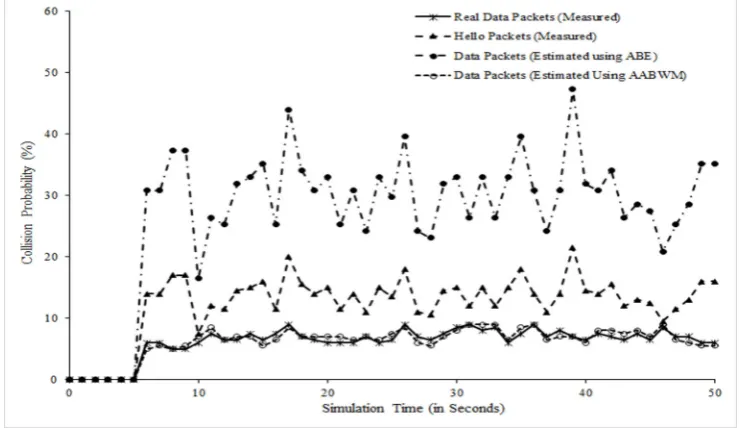
To calculate the collision probability the authors in [4] make use of the HELLO packets. A counter was deployed at the receiver end to count the number of HELLO packets that are received at the destination in real time. The collision probability of HELLO packets is calculated by dividing the value of the above counter by the actual number of the HELLO packets that should have been received in idealized conditions. Since the size of the HELLO packets is small in comparison to the data packets the above results are interpolated to predict the collision probability of data packets. However, there are several drawbacks attached to this process. It can be observed from Fig. 3.3 that the estimated values of data packet collisions are far away from the real values of data packets collisions measured using NS2. This over-evaluation is because HELLO packets which are delayed or lost due to network congestion or overloaded medium are combined with the collision rate of HELLO packets and further interpolating the same overvalued its effect. This revealed the abortive behavior of [4] approach for the computation of collision probability.

To overcome the computation failure existing due to passive technique proposed in [4], our work uses an analytical approach using fixed-point analysis (FPA) based on renewal theory for the calculation of collision probability. The proposed solution is influenced by [17]. The main assumption being ideal channel conditions. The only reason for the unsuccessful packet transmission is the collision of packets. It is also assumed that all stations use the different backoff parameter thus having different collision probability (pl) and attempt rate (or transmission probability) (τl) where l=1, 2... n. Letnbe the number of contending nodes, the attempt bylth

node is successful if all other contending nodes are silent. Mathematically, it can be written as: 1−pl=∏

j̸=l

(1−τj);f orj, l= 1,2, ..., n

Fig. 3.3.Estimated results of collision probabilities of packets.

Let qdenotes the probability of a non-empty buffer, i.e. at least one packet is available for transmission after transmitting the current one. According to [17] the attempt rate of a node in non-saturated network condition can be obtained by scaling down the attempt rate of a node in saturated condition with the probability of non-empty buffer. Thus, we have

τl=q.τls

(3.6)

where τls represent the lth _{node’s attempt rate (or probability) under saturated network conditions. To solve}

the fixed-point equation given by (3.5) and (3.6), there is a need to expressτli.e. qandτls) in terms of collision probability (pl).

The attempt rate of a node in saturated condition (τls) is defined as the ratio of average number of attempts to the average number of backoff time (in slots) spent by a node till the successful transmission of the packet. According to [16], we have:

τls=f(p) = E[attempts]

E[backof f] (3.7)

where the average attempt rate is given as:

E[attempts] = 1 +pl+pl2+...+plm

(3.8)

According to IEEE 802.11 standard whenever a packet suffers collision, the exponential backoff mechanism is triggered; the backoff associated with the initial transmission attempt by a node is b0 and it is doubled after every unsuccessful attempt till the maximum limitmis reached. The average backoff time per packet is given as:

E[backof f] =b0+pl(2b0) +...+plm′(2m′b0) +...+plm(2m′b0) (3.9)

where

b0=

CW0is the minimum contention window size = 31 slots. And,m′ _{represent a constant where contention window}

size reaches its maximum valueCWmax, represented as:

CWmax= 2m′CW0

(3.11)

Thus, using (3.5) and (3.6) we get,

τl= q.(1 +pl+pl

2_+...+plm₎ b0+pl(2b0) +...+plm′

(2m′

b0) +...+plm₍₂m′ b0) (3.12)

For simplicity of expression we assumed Poisson traffic arrival rate, however the solution is equally applicable to other traffic arrival types also such as Constant Bit Rate (CBR), exponential on/off traffic and Pareto on/off traffic. Using queuing theory, the traffic intensityρis given as:

ρ=ρ(λ, p) =λ.ST

(3.13)

whereλis packet arrival rate,ST is a mean service time of a packet which is dependent on the average backoff time i.e. E[backoff] waiting till the successful transmission of the packet and the average slot timeEsdepending on the channel activity i.e. idle slot time, successful attempt and collision occurrence. Thus, (3.13) can be re-written as:

ρ=λ.E[backof f].Es

(3.14)

The average time Esspent per slot is given as:

Es= (1−Ptr)σ+PtrPsiTsi+Ptr(1−Psi)Tci

(3.15)

where Ptr represent the probability that at least one transmission going on in the network; σis the slot time andPsi represents the probability that the transmission byithstation is successful.

Ptr= 1−

n

∏

i=1(1−τj)

(3.16)

Psi =τi

∏

j̸=1

(1−τj) (3.17)

Tsi andTci represent the expected time for successful transmission and unsuccessful transmission respectively.

These transmission times are governed by the access mechanism employed i.e. Basic access mechanism and RTS/CTS access mechanism.

T_sbasici =DIF S+T(H+DAT A)+SIF S+TACK

(3.18)

Tcbasici =DIF S+T(H+DAT A)+ACKtimeout

(3.19)

TsRT S/CT Si =DIF S+TRT S+SIF S+TCT S+SIF S

+T(H+DAT A)+SIF S+TACK

(3.20)

T_cRT S/CT Si =DIF S+TRT S+CT Stimeout

(3.21)

where DIFS is Distributed Inter-Frame Space time; SIFS is Short Inter-Frame Space time; TRT S, TCT S, and

TACK are the time required for RTS, CTS, and ACK control packet transmission respectively;T(H+DAT A)is the

and ACKtimeout are the waiting time required before declaring unsuccessful transmission for RTS and DATA packet respectively.

To solve (3.12), the value of qneeds to be determined. The probability of non-empty buffer is dependent on the node’s buffer size as well as offered load. We have taken two extreme cases of buffer sizes to evaluate the value ofq; one for small buffer and another for infinite buffer. This is expressed by [17] as:

q=1−e−ρ; for small buffer model

min(1, ρ); for infinite buffer model

(3.22)

Substituting the value of q from (3.22) in (3.12), we get the following equations under two different cases as considered:

Case-I: Small Buffer case

τl= (1−e

−ρ_{).(1 +pl+pl}2_+...+plm₎

b0+pl(2b0) +...+plm′

(2m′

b0) +...+plm₍₂m′ b0) (3.23)

Case-II: Infinite Buffer case

τl= (min(1, ρ)).(1 +pl+pl

2_+...+plm₎ b0+pl(2b0) +...+plm′₍₂m′

b0) +...+plm₍₂m′ b0) (3.24)

Solving the coupled nonlinear equations (3.5) and (3.23) provide the precise estimation of collision probability

pland the attempt rateτlof thelth_node.

3.3. Special case for Homogeneous Network Model. Consider homogeneous network conditions where all stations are having same backoff parameters. Letn be the number of stations in the network, then average attempt rateτand collision probabilitypof each station are same. Under the decoupling approximation, the probability of collision pof an attempt by a node is obtained by reducing the equations mentioned in Sec. 3.2 as:

1−p= (1−τ)n−1 (3.25)

The expected time spent per state reduces to:

Es= (1−Ptr)σ+nPsTs+ (Ptr−nPs)Tc

(3.26)

where, the probability of successful transmissionPsof any sending station is given by: Ps=τ(1−τ)n−1

(3.27)

The probability Ptr that at least one transmission is going on in the network reduces to:

Ptr = 1−(1−τ)n (3.28)

The probability of non-empty buffer under homogeneous network condition is obtained by re-writing (3.23) and (3.24). Thus, we have:

Case-I: Small Buffer case

τ= (1−e

−ρ_{).(1 +p+p}2_+...+pm₎

b0+p(2b0) +...+pm′₍₂m′_{b0) +...+p}m₍₂m′_b0)

(3.29)

Case-II: Infinite Buffer case

τ= (min(1, ρ)).(1 +p+p

2_+...+pm₎ b0+p(2b0) +...+pm′

(2m′

b0) +...+pm₍₂m′ b0) (3.30)

3.4. Bandwidth consumed due to backoff mechanism . Whenever a packet transmission occurs between sender and receiver node, the packets may suffer collision at sender s or receiver node r. In both cases the exponential backoff mechanism is triggered at sender node. The time lost due to backoff mechanism is not used for transmitting the packet, even if the medium is idle. Thus, a proportion of idle time wasted due to backoff mechanism having a significant impact on the ABW. The average backoff time associated with the collision probability pl is obtained using (3.9). Thus, the loss of local ABW of sender node due to backoff mechanism can be mathematically represented as given in [19]:

LocalABWs=

(ts−E[backof f])

T Cmax

(3.31)

wheretsis the idle time of sender(s) obtained using (3.1) and E[backoff] is the average backoff time calculated using (3.9) andCmax is the raw channel capacity.

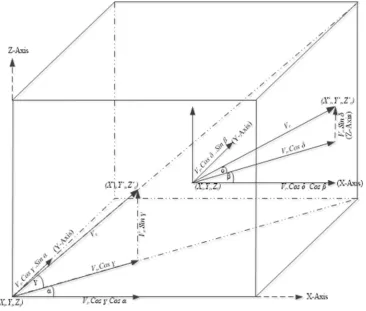
3.5. Link Prediction Factor in 3-Dimensional space . Mobility causes the frequent link breakage and re-construction leading to delay and data losses which eventually impact the ABW. Limited literature is available on the issue of mobility while calculating the available bandwidth. Most of the work addressing the mobility has considered two dimensional space only. The current work predicts the link expiration caused due to mobility of nodes under 3-dimensional space. The approach is equally applicable to all channel environments. Fig. 3.4 represents the 3-dimensional mobility model for the movement of sender and receiver nodes. Let the initial position of sender station and receiver station be (Xs, Ys, Zs) and (Xr, Yr, Zr) respectively. Sender station is moving in 3-dimensional world with velocityVsmaking an angleγwith z-direction and angleαwith x-direction. AsVs is making an angle ofγ in z-direction, the vector component ofVs in X-Y plane isVs.cosγ

and vector component of Vs in z-axis is Vs.sinγ. Further, as the angle with respect to x-direction is α, the vector component of Vs.cosγin x-axis isVs.cosγ.cosαand in y-axis isVs.cosγ.sinα.

Receiver station is moving in 3-dimensional world with velocity Vr making an angleδwith z-direction and angle β with x-direction. As Vr is making an angle of δ in z-direction, the vector component of Vr in X-Y plane will be Vr.cosδ and vector component of Vr in z-axis is Vr.sinδ. Further, as the angle with respect to x-direction is β, the vector component ofVs.cosδin x-axis isVs.cosδ.cosβ and in y-axis isVs.cosδ.sinβ.

After time t let the coordinates of sender station and receiver station are (Xs, Ys, Zs) and (Xr, Yr, Zr) respectively. The new coordinates of the sender and receiver station can be mathematically written as:

X′s=Xs+tVscosγcosα

(3.32)

Y′s=Ys+tVscosγsinα

(3.33)

Z′s=Zs+tVssinγ

(3.34)

X′r=Xr+tVrcosδcosβ

(3.35)

Y′r=Yr+tVrcosδsinβ

(3.36)

Z′r=Zr+tVrsinδ

(3.37)

Therefore, the distance between sender and receiver after timetin X, Y and Z directions can be determined as:

X′

s−X′r= (Xs−Xr) +t(Vscosγcosα−Vrcosδcosβ)

(3.38)

Y′s−Y′r= (Ys−Yr) +t(Vscosγsinα−Vrcosδsinβ)

Fig. 3.4.3-Dimensional reference model.

Z′s−Z′r= (Zs−Zr) +t(Vssinγ−Vrsinδ)

(3.40)

Let the vector distance between sender and receiver after time t be D. Then, using Pythagoras Theorem the

D can be calculated as:

D2= (X′s−X′r)2+ (Y′s−Y′r)2+ (Z′s−Z′r)2

(3.41)

Substituting the values from (3.38), (3.39) and (3.40) in (3.41), we get

D2= = ((Xs−Xr) +t(Vscosγcosα−Vrcosδcosβ))2 + ((Ys−Yr) +t(Vscosγsinα−Vrcosδsinβ))2 + ((Zs−Zr) +t(Vssinγ−Vrsinδ))2

(3.42)

This can be re-written as:

D2= (a+tf)2+ (b+tg)2+ (c+th)2 (3.43)

wherea=Xs−Xr,b=Ys−Yrandc=Zs−Zrare the initial distance between sender and receiver station in X, Y and Z directions respectively. The relative velocity component between the two in X, Y and Z directions respec-tively can be mathematically expressed as f =Vs.cosγ.cosαVr.cosδ.cosβ, g = Vs.cosγ.sinαVr.cosδ.sinβ;

andh=Vs.sinγVr.sinδ. Solving (3.43) for the value of timet, we get:

t=−(af+bg+ch)± √

(f2_+g2_+h2_).D2_−(ag−bf)2_−(bh−gc)2_−(ah−cf)2

(f2_+g2_+h2₎

Global positioning system in [21] facilitates the coordinate’s information. With each Hello packet, station broadcasts starting and terminus coordinates along with its velocity. The sender station, receiving the hello packet from receiver station evaluates the link availability time durationtand thereby the mobility factorM M.

M M= t

T

(3.45)

whereT is the measurement period,tis the duration for which the sender-receiver stations are within commu-nication range.

The final ABW on a link(s,r) constituting between sender s and receiverr is computed by combining all the major factors discussed in the sub-sections of the current section (i.e. Sec. 3) of this paper. The final ABW estimated on link(s,r) is given as:

ABWAABW M = (

ts−E[backof f]

T .

tr

T.Cmax)(1−pl)(M M)

(3.46)

wheretsandtrrepresent the sum of idle times sensed at sender and receiver node respectively computed using (3.1) during measurement periodT; E[backoff] represent the local ABW wasted at the sender node as given by (3.9); Cmax is the maximum channel capacity; pl represents the collision probability of data packets as driven in Sec. 3.2 obtained by solving (3.5) and (3.23) or (3.24); and a M M link persistence factor representing the mobility effect of nodes in 3-dimensional space is given in (3.46).

3.6. Throughput efficiency (S). Saturation throughput of a system is defined as the maximum data that the system can transfer successfully under steady state conditions. Mathematically, the throughputS of a system can be expressed as the summation of each individual source station’s throughput efficiency.

S=∑n

i=1Si

(3.47)

whereSi represents the throughput efficiency ofith_{source station,i∈[1, n] andnis the total number of source}

stations in the network. The throughput efficiency of the individual source station can be calculated as the fraction of the time used by source station for successfully transferring the payload information and is expressed as:

Si= PsiLi

Es

(3.48)

where Psi represents the probability that the transmission byithstation is successful and is derived in (3.17);

Liis the time taken to transmit payload data byithsource station; andEsis the expected time spent per state as derived in (3.15).

3.7. Protocol Design. To provide comparative analysis and visualizing the impact of mobility factor in (3.46), our proposed approach AABWM employs AODV [22] as routing protocol. Assuming a node having data to transmit. It first determines it’s local ABW using (3.1) based on idle/busy periods sensed by the node by monitoring the radio channel activities. If it’s local ABW is enough for the flow transmission, it broadcasts a route request packet (RREQ) consisting of the required bandwidth for its flow. All the nodes within its range receive this RREQ packet, and perform admission control by comparing the required bandwidth within the RREQ packet with the computed ABW using (3.46) on the link composed with its fore goer node. If bandwidth is enough, then node combines its own information with the fore goer and forwards the RREQ packet otherwise drop the packet. When the intended destination node receives the packet, it reverts with the uni-cast RREP (route reply packet) packet to the initiator along with the reverse path.

If the bandwidth estimation is done after admitting the flow and link has no enough bandwidth then the node sends a route error packet (RERR) to the initiator. On receiving the RRER packet, the initiator takes immediate action to prevent the losses and stops the ongoing transmission.

Table 4.1

Simulation parameters values for comparative analysis

Raw channel capacity 2 Mbps Topology size 700x700x700 meter Routing protocol AODV Medium access protocol CSMA Packet size 1000 Bytes Transmission range 250 m Carrier sensing range 550 m

Simulation time 100 seconds Flow-1 CBR 250 kbps Flow-2 CBR 500 kbps Flow-3 CBR 400 kbps Flow-4 CBR 550 kbps Flow-5 CBR 450 kbps Flow-6 CBR 300 kbps Minimum contention window (CWmin) 31 slot

Maximum contention window (CWmax) 1023 slot

Maximum retry limit (m) 6

Fig. 4.1.Throughput of flows using AODV [22] without any admission control.

4.1. Simulation Scenario. A network consists of 48 nodes randomly distributed over a small area (700m x 700m x 700m) is considered. Six CBR single-hop flow connections (Flow-1 to Flow-6) are established. Each flow is having a different transmission rate to make the network heterogeneous. The parameters used for simulation are derived from IEEE 802.11b and are listed in Table 4.1.

4.2. Simulation results and Comparative Analysis. The comparative analysis is split into two cases: a) Case-I, consists of stationary nodes to evaluate the accuracy of our proposed approach AABWM with the traditional approaches; and b) Case-II, consists of mobile nodes which are free to move in 3-dimensional space, thereby giving us an opportunity to visualize its effect on link persistence and thus on the admission control.

Case-I: Considering no mobility of nodes

Flows 1 to 6 are generated at an interval of 10 seconds starting fromt= 5 second. Fig. 4.1 to Fig. 4.5 plots the throughput of six flows obtained when AODV [22], ABE [4], IAB [7], IBEM [18] and AABWM approaches are activated respectively.

In AODV [22], all flows are admitted as no admission control is employed. However, with the introduction of flow-4(550kbps) at a time,t=35s channel capacity is reached; the performance of existing flows gets deteriorated. The throughput further got worse by the introduction of flow-5(450kbps) and flow-6(300kbps).

Fig. 4.2.Throughput of flows using ABE [4] for admission control.

Fig. 4.3.Throughput of flows using IAB [7] for admission control.

ABE [4]. The system resources are not optimally utilized, the total system throughput is far below maximum channel capacity. This underestimation of ABW is due to the bad computation of collision probability and assimilates the same in bandwidth estimation.

In IAB [7], over-estimation of ABW takes place, thereby allowing flow-4(550kbps) which leads the channel congestion and all existing flows got suffered in terms of throughput performance. Due to collisions arising from network congestion, a lot of bandwidth got wasted; thereby degrading overall system performance. However, flow-5(450kbps) and flow-6(300kbps) are rejected as ABW estimated using IAB [7] is not enough for these flows. Fig. 4.4 represent the throughput of six flows along the simulation duration when IBEM approach is enabled. To calculate the collision probability IBEM assumed the saturated condition as in [19] and ignore the empty state of nodes buffer. Thus, overestimating the impact of collisions leading to underestimate the ABW; thereby admission of flows (flow-4 and flow-5) is not permitted. Further, Flow-6(300kbps) is accepted as ABW estimated using IBEM is enough for this flow.

Fig. 4.4.Throughput of flows using IBEM [18] for admission control.

Fig. 4.5.Throughput of flows using proposed AABWM for admission control.

Case-II: Considering the 3-Dimensional mobility of nodes

To visualize the impact of mobility of nodes, the Random way point mobility model is used in the 3-dimensional space to assign random movement to the nodes with random direction and velocity. Initially the flows 1 to 6 are generated at random time interval. The start and stop of flows are automated by the admission control protocol depending on the ABW estimation technique employed. The simulation results obtained using AODV [22], ABE [4], IAB [7], IBEM [18] and AABWM under the influence of 3-dimensional movement of nodes is represented in Fig. 4.6 to Fig. 4.10.

Fig. 4.6 represents the throughput of all flows when the AODV [22] routing protocol is enabled. Absence of any admission control in AODV [22], all flows are admitted leading to high network congestion and increased collisions. There is no QoS guarantee given to any flow, even the flows having a shorter duration of link existence (Flow-4 and Flow-5) is allowed causing a lot of bandwidth and data loss.

Fig. 4.7 depicts the throughput of all six flows when ABE [4] approach is activated. Inability of ABE [4] to predict link failure caused due to mobility permit the admission of short persisted flow-4(550kbps) at time

t=10s and flow-5(450kbps) att=15s. Although the admitted flows are less in ABE [4] as compared to AODV [22] and flow’s throughput are also stable, but still due to false admission of flows (Flow-4 and Flow-5) the network resource is not adequately utilized. Incomplete transmission due to link failure causes loss of data and thus the bandwidth.

Fig. 4.6.Throughput of flows using AODV [22] without any admission control.

Fig. 4.7.Throughput of flows using ABE [4] for admission control.

network congestion by allowing short lived flows such as flow-4(550kbps) att=25s and flow-5(450kbps) att=55s despite of non-availability of enough ABW leading to performance degradation of existing flows. We observed poor individual flow’s throughput performance and a lot of data packets loss in this scenario due to higher collisions.

Fig. 4.9 depicts the throughput of the flows when IBEM [18] approach is enabled. IBEM restricted its study to 2-dimensional plane only and ignored the movement of nodes under 3-dimensional space. Thus, it predicts the link failure of flow-5(450kbps) att=15s and not allowed it to admit at this instance. IBEM admitted short lived flows (flow-4 at t=10s and flow-5 at t=85s) due to the inability to predict link failure at 3-dimension leading to data losses. Moreover, the admission of flow-3(400kbps) is delayed and started at t=25s due to false admission of flow-4(550kbps). IBEM performed better than earlier approaches, but still admission control is severe in this due to ignoring the effects of elevation and height while predicting the link failure.

Fig. 4.10 shows the received throughput when AABWM is enabled. Short lived flow-4 at (t=10s and

Fig. 4.8.Throughput of flows using IAB [7] for admission control.

Fig. 4.9.Throughput of flows using IBEM [18] for admission control.

4.3. Packet Loss Ratio. The packet loss ratio is defined as the ratio of the number of data packets lost to the number of data packets sent by the sender. The number of lost data packets is calculated as the difference of the number of packets sent by the sender and the number of packets received at receiver node. Mathematically, this can be written as:

Packet Loss ratio=number of sent packets−number of received packets

number of sent packets by the sender

(4.1)

Fig. 4.11 depicts the packet loss ratio measured under the effect of mobility in the above experiment using NS2. We observe the packet loss ratio is negligible for all flows when AABWM is incorporated in admission control protocol. Whereas, other techniques resulting in an elevated packet loss ratio for flow 1 to 6.

4.4. Data Packets Delivery. The data packets delivery is calculated as the total number of data packets received at receiver node. The data packets delivery does not necessarily mean the useful data, rather it represents the total number of data packets delivered irrespective of the communication is completed. Fig. 4.12 represents the data packets delivery under the influence of node’s mobility.

Fig. 4.10. Throughput of flows using proposed AABWM approach for admission control.

Fig. 4.11.Packet loss ratio.

Chain based solutions. The link failure due to mobility of nodes leads to wastage of bandwidth resources and needs to be addressed while evaluating the available bandwidth. We incorporate the mobility issue and observed that link failure due to mobile nodes adversely affect the bandwidth estimation efforts. The proposed model is compared against the existing approaches in terms of bandwidth consumption and admission control solution using ns-2 simulations. The results indicate that in both static environment and dynamic environment the proposed model has most stable performance. The packet loss ratio is found to be least in comparison to other algorithms. The increased value of packet delivery ratio indicates the improvement in terms of delivery and throughput achieved by the proposed solution.

REFERENCES

[1] C. Chaudet, and I. Gurin Lassous,BRuIT: Bandwidth Reservation under InTerference Influence, European Wireless (EW 02), Florence, Italy, 2002, pp. 466–472.

[2] Y. Yang, and R. Kravets, Contention-Aware Admission Control for Ad hoc Networks, IEEE Transactions on Mobile Computing, 4 (2005), pp. 363–377.

[3] R. de. Renesse, V. Friderikos, and H. Aghvami,Cross-layer cooperation for Accurate Admission Control Decision in Mobile Ad hoc Networks, IET Communications, 1 (2007), pp. 577–586.

[4] C. Sarr, G. Chaudet, G. Chelius, and I. G. Lassous,Bandwidth Estimation for IEEE 802.11-Based Ad hoc Networks, IEEE Transactions on Mobile Computing, 7 (2008), pp. 1228–1241.

[5] C. Dovrolis, P. Ramanathan, and D. Moore,What do Packet Dispersion Techniques Measure?, Proc. IEEE INFOCOM, 2001, pp. 905–914.

[6] Y. Xiao, S. Chen, X. Li, and Y. Li,A New Available Bandwidth Measurement Method Based on Self-Loading Periodic Streams, in Wireless Communications, Networking and Mobile Computing, Shanghai, China, 2007, pp. 1904–1907. [7] H. Zhao, E. Garcia-palacios, J. Wei, and Y. Xi,Accurate Available Bandwidth Estimation in IEEE 802.11-based Ad Hoc

Networks, Computer Communications, 32 (2009), pp. 1050–1057.

[8] S. S. Chaudhari, and R. C. Biradar,Collision Probability based Available Bandwidth Estimation in Mobile Ad Hoc Net-works, Applications of Digital Information and Web Technologies (ICADIWT), 2014, pp. 244–249.

[9] G. Bianchi,Performance Analysis of the IEEE 802.11 Distributed Coordination Function, IEEE Journal on Selected Area in Communication, 18 (2000), pp. 535–547.

[10] H. Wu, Y. Peng, K. Long, S. Cheng, and J. Ma,Performance of Reliable Transport Protocol over IEEE 802.11 Wireless LAN: Analysis and Enhancement, Proc. IEEE INFOCOM’02, 2 (2002), pp. 599–607.

[11] P. Chatzimisios, A. C. Boucouvalas, and V. Vitas,Performance Analysis of the IEEE 802.11 MAC protocol for Wireless LANs, International Journal of Communication Systems, 18 (2005), pp. 545–569.

[12] E. Ziouva, and T. Antonakopoulos, CSMA/CA Performance under High Traffic Conditions: Throughput and Delay Analysis, Computer Communications, 25 (2002), pp. 313–321.

[13] C. H. Foh, and J. W. Tantra, Comments on IEEE 802.11 Saturation Throughput Analysis with Freezing of Backoff Counters, IEEE Communication Letters, 9 (2005), pp. 130–132.

[14] Y. S. Liaw, A. Dadej, and A. Jayasuriya,Performance Analysis of IEEE 802.11 DCF under Limited Load, Proc. Asia-Pacific Conference on Communications, 2005, pp. 759–763.

[15] D. Malone, K. Duffy, and D. Leith,Modeling the 802.11 Distributed Coordination Function in Nonsaturated Heterogeneous Conditions, IEEE/ACM Transactions on Networking, 15 (2007), pp. 159–172.

[16] A. Kumar, E. Altman, D. Miorandi, and M. Goyal,New Insights from a Fixed Point Analysis of Single Cell IEEE 802.11 WLANs, Proc. IEEE INFOCOM, 2005, pp. 1550–1561.

[17] Q. Zhao, D.H.K. Tsang, and T. Sakurai,A Simple and Approximate Model for Nonsaturated IEEE 802.11 DCF, IEEE Transactions on Mobile Computing, 8 (2009), pp. 1539–1553.

[18] R. Belbachir, Z. M. Maaza, and A. Kies,The Mobility Issue in Admission Controls and Available Bandwidth Measures in MANETs, Wireless Personal Communications, 70 (2013), pp. 743–757.

[19] R. Belbachir, Z. M. Maaza, A. Kies, and M. Belhadri,Collision’s Issue: Towards a New Approach to Quantify and Predict the Bandwidth Losses, Global Information Infrastructure Symposium, Trento, Italy, 2013, pp. 1–7.

[20] L. Chen, and W.B. Heinzelman,QoS-Aware Routing based on Bandwidth Estimation for Mobile Ad Hoc Networks, IEEE Journal on Selected Areas in Communications, 23 (2005), pp. 561–572.

[21] E. Kaplan, and C. Hegarty,Understanding GPS: Principles and Applications, Artech House, 2005.

[22] C. Perkins, E. Belding-Royer, and S. Das,Ad hoc On-Demand Distance Vector (AODV) Routing, RFC Editor, 2003.