R E S E A R C H
Open Access
Analysis and application of the discontinuous
Galerkin method to the RLW equation
Jiˇrí Hozman
1*and Jan Lamaˇc
1,2*Correspondence: [email protected]
1Faculty of Science, Humanities and Education, Technical University of Liberec, Studentská 2, Liberec, 461 17, Czech Republic
Full list of author information is available at the end of the article
Abstract
In this work, our main purpose is to develop of a sufficiently robust, accurate and efficient numerical scheme for the solution of the regularized long wave (RLW) equation, an important partial differential equation with quadratic nonlinearity, describing a large number of physical phenomena. The crucial idea is based on the discretization of the RLW equation with the aid of a combination of the discontinuous Galerkin method for the space semi-discretization and the backward difference formula for the time discretization. Furthermore, a suitable linearization preserves a linear algebraic problem at each time level. We present error analysis of the proposed scheme for the case of nonsymmetric discretization of the dispersive term. The appended numerical experiments confirm theoretical results and investigate the conservative properties of the RLW equation related to mass, momentum and energy. Both procedures illustrate the potency of the scheme consequently.
PACS Codes: 02.70.Dh; 02.60 Cb; 02.60.Lj; 03.65.Pm; 02.30.-f
MSC: 65M60; 65M15; 65M12; 65L06; 35Q53
Keywords: discontinuous Galerkin method; regularized long wave equation; backward Euler method; linearization; semi-implicit scheme;a priorierror estimates; solitary and periodic wave solutions; experimental order of convergence
1 Introduction
We are concerned with a proposal of a sufficiently robust, accurate and efficient numeri-cal method for the solution of snumeri-calar nonlinear partial differential equations. As a model problem, we consider a regularized long wave (RLW) equation firstly introduced by Pere-grine (in []) to provide an alternative description of nonlinear dispersive waves to the Korteweg-de Vries (KdV) equation. As a consequence of this, the RLW can be observed as a special class of a family of KdV equations.
The RLW equation contains a quadratic nonlinearity and exhibits pulse-like solitary wave solutions or periodic waves; see []. It governs various physical phenomena in disci-plines such as nonlinear transverse waves in shallow water, ion-acoustic waves in plasma or magnetohydrodynamics waves in plasma. Since the RLW equation can be solved by analytical means in special cases, the proposed numerical methods can be easily verified. Several numerical studies of the RLW equation and its modified variant have been intro-duced in the literature, from finite difference methods [], over collocation methods [, ], to finite element approaches [, ], or Galerkin methods [], and in references cited therein.
In this paper, we present a semi-implicit scheme for the numerical solution of the RLW equation based on an alternative approach to the commonly used methods. The discon-tinuous Galerkin (DG) methods have become a very popular numerical technique for the solution of nonlinear problems. DG space semi-discretization uses higher-order piecewise polynomial discontinuous approximation on arbitrary meshes; for a survey, see [, ] and []. Among several variants of DG methods, we deal with the nonsymmetric variant inte-rior penalty Galerkin discretizations; see []. The discretization in time coordinate is per-formed with the aid of linearization and the backward Euler method, sidetracking the time step restriction well known from the explicit schemes, proposed in []. Consequently, we extend the results from [], and the attention is paid to thea priorierror analysis of the method with the aid of standard techniques introduced in [] and [].
The rest of the paper is organized as follows. The problem formulation and its variational reformulation are given in Section . Discretization, including space semi-discretization and fully time space discretization, is considered in Section . The Section is devoted toa priorierror analysis. Finally, in Section , the theoretical results are illustrated by numeri-cal tests on a propagation of a single solitary wave and experimental orders of convergence are computed for piecewise linear approximations together with invariant quantities of the RLW equation.
2 Regularized long wave equation
Let= (a,b)⊂Rbe a bounded open interval andT > be a final time. We setQT=
×(,T) and consider the following initial boundary value problem: Findu(x,t) :QT=
×(,T)→Rsuch that, for allT> ,
∂u ∂t +
∂u ∂x +εu
∂u ∂x–μ
∂ ∂t
∂u ∂x
= inQT, ()
u(a,t) =uaD(t) and u(b,t) =ubD(t) for allt∈(,T), ()
u(x, ) =u(x) for allx∈, ()
where constant parametersε> andμ> are related to the amplitude of the wave and long-wavelength, respectively. From the mathematical point of view, problem ()-() rep-resents the regularized long wave equation equipped with a set of two generally nonho-mogeneous Dirichlet boundary conditions () and with the initial conditionu:→R.
These given data have to satisfy the compatibility conditions prescribed at both endpoints of the domain,i.e.,
uaD() =u(a) and ubD() =u(b). ()
The whole system ()-() was found to have single solitary or periodic traveling wave so-lutions; for details, see [].
In what follows we use the standard notation for function spaces and their norms · and seminorms | · |. Let k≥ be an integer and p∈[,∞]. We use the well-known Lebesgue and Sobolev spacesLp(),Hk(), Bochner spacesLp(,T;X) of functions de-fined in (,T) with values in a Banach spaceXand the spacesCk([,T];X) ofk-times continuously differentiable mappings of the interval [, T] with values inX. ByH
() we
denote the subspace of all functionsv∈H() satisfyingv(a) =v(b) = . To this end, we
use the following notation for a scalar product inL() by
(u,v) =
uvdx, u,v∈L() ()
for a norm inL() by · =
√
(·,·), for a seminorm inH() by| · |,=
√
(∇·,∇·) and for a norm inH() by ·
,=
√
(·,·) + (∇·,∇·). It is a known fact that| · |,is a norm on H() equivalent to · ,
A sufficiently regular solution satisfying ()-() pointwise is called aclassical solution. Now, we are ready to introduce the concept of weak formulation. Firstly, we recall the definition of a bilinear dispersion forma(·,·) and a nonlinear convection formbε(·,·) from [],i.e.,
au(t),v=
∂u(t)
∂x ·v
dx, ()
bεu(t),v=
∂f(u(t))
∂x ·vdx withf(u) =u+ ε
u
, ()
where symbolu(t) stands for the function onsuch thatu(t)(x),x∈and functionf(u) in () represents the physical flux.
Definition We say thatuis a weak solution of problem ()-() ifu∈L(,T;H())∩
L∞(QT) such that ∂∂ut ∈L(,T;H()) and the following conditions are satisfied:
(a) u–u∗∈L,T;H(), whereu∗(t)∈H() such that
u∗(t)|x=a=uaD(t) andu∗(t)|x=b=ubD(t) for a.e.t∈(,T),
(b) d dt
u(t),v+bεu(t),v+μd
dta
u(t),v= ∀v∈H() and a.e.t∈(,T),
(c) u(),v=u,v ∀v∈H(),u∈L().
()
Remark In order to unify the definition of the weak solution (), we consider
nonhomo-geneous Dirichlet boundary conditions instead of the second parallel analysis of periodic-type solutions with the aid of Sobolev spaces of periodic functionsHk
λ((a,b)) with period
λ> satisfyingmod(b–a,λ) = .
Assumptions (R)
(R) u,∂u
∂t ∈L
∞,T;Hs+(), s≥, ()
(R) ∂
u
∂t ∈L
∞,T;H(), ()
(R) ∂u(t)
∂x
L∞()
≤CD for a.a. t∈(,T). ()
3 Discretization
LetTh(h> ) be a family of the partitions of the closure= [a,b] of the domaininto
N closed mutually disjoint subintervalsIk= [xk–,xk] with lengthhk:=xk–xk–and the
symbolJ stands for an index set{, . . . ,N}. Then we callTh={Ik,k∈J}a partition with a spatial steph:=maxk∈J(hk) and intervalIk an element. ByEh we denote the set of all partition nodes of,i.e.,Eh={x=a,x, . . . ,xN–,xN=b}. Further, we label byEhI the set of all inner nodes. Obviously,Eh=EhI∪ {a,b}.
We additionally assume that the partitions satisfy the following condition.
Assumption (M) Thare locally quasi-uniform:
∃Cq≥ :hk≤Cqhk ∀Ik,Ik∈Thsharing a node. ()
The condition () in fact allows to control a level of the mesh refinement if adapted meshes are used.
DG methods can handle different polynomial degrees over elements. Therefore, we as-sign a local Sobolev indexsk∈Nand a local polynomial degreepk∈Nto eachIk∈Th. Then we set the vectorss≡ {sK,K∈Th}andp≡ {pK,K∈Th}. Over the triangulationTh, we define the so-called broken Sobolev space corresponding to the vectorsas
Hs(,Th) :=
v;v|Ik∈H sk(I
k)∀Ik∈Th ()
with the norm
vHs(,T
h):= Ik∈Th
vHsk(Ik)
/
()
and the seminorm
|v|Hs(,T
h):= Ik∈Th
|v|Hsk(Ik)
/
, ()
where·Hsk(Ik)and|·|Hsk(Ik)denote the standard norm and the seminorm on the Sobolev spaceHsk(I
k),Ik∈Th.
The approximate solution of variational problem () is sought in a finite dimensional space of discontinuous piecewise polynomial functions associated with the vectorpby
Shp≡Shp(,Th) :=
v;v|Ik∈Ppk(Ik)∀Ik∈Th , ()
Let us denotev(x+k) =limε→+v(xk+ε) andv(x–k) =limε→+v(xk–ε). Then we can define the jump and average ofvat inner pointsxk∈EhI of the domainby
v(xk)
=vx–k–vx+k, v(xk)
=
vx–k+vx+k. ()
By convention, we also extend the definition of jump and mean value for endpoints of,
i.e., [v(x)] = –v(x+),v(x)=v(x+), [v(xN)] =v(x–N) andv(xN)=v(x–N). In case thatxk∈Eh are arguments ofv(x–k) orv(x+k), we usually omit these argumentsx–k,x+kand write simply
v–andv+, respectively.
3.1 DG semi-discrete formulation
Now, we recall the space semi-discrete DG scheme presented in []. First, we multiply () by a test functionvh∈Shp, integrate over an elementIk∈Thand use integration by parts in the dispersion termahand convection termbεhof () subsequently. Further, we sum over allIk∈Th and add some artificial terms vanishing for the exact solution such as penalty
Jσ
h and stabilization terms, which replace the inter-element discontinuities and guarantee the stability of the resulting numerical scheme, respectively. Consequently, we employ the concept of an upwind numerical flux (see []) for the discretization of the convection term and end up with the following DG formulation for the semi-discrete solutionuh(t), introduced in [] as a system of ordinary differential equations,i.e.,
d dt
uh(t),vh
+μah
uh(t),vh
+μJhσuh(t),vh +bεh
uh(t),vh
=
∀vh∈Sh,∀t∈(,T), ()
where formsah(·,·) andbεh(·,·) stand for the semi-discrete variants of forms () and (),
i.e.,
ah
u(t),v= k∈J
Ik
∂u(t)
∂x ·v
dx–
x∈Eh
∂u(t)
∂x
[v] + x∈Eh
vu(t), ()
bεhu(t),v= – k∈J
Ik
u+ε u
·vdx+ x∈Eh
Hu–(t),u+(t)[v]. ()
The crucial item of the DG formulation of the model problem is the treatment of the convection part. We proceed analogously as in [], where the convection terms are ap-proximated with the aid of the following numerical fluxH(·,·) through nodex∈Ehin the positive direction (i.e., outer normal is equal to one):
Hux–,ux+=
⎧ ⎨ ⎩
f(u(x–)) =u(x–) +εu(x–), ifA> ,
f(u(x+)) =u(x+) +ε
u(x+), ifA≤,
()
whereA=f(u(x–)+u(x+)) and the choice off(u(x–
)) andf(u(x+N)) for boundary points has to satisfy the prescribed Dirichlet boundary conditions; for more details, see [].
In what follows, we shall assume that the numerical fluxH:R→Rhas the following
Assumptions (H)
(H) H(u,v)is Lipschitz-continuous with respect tou,v:
H(u,v) –Hu∗,v∗≤CHu–u∗+v–v∗, u,v,u∗,v∗∈R. ()
(H) H(u,v)is consistent:
H(u,u) =f(u), u∈R. ()
(H) H(u,v)is conservative:
H(u,v) = –H(v,u) in the negative direction,u,v∈R. ()
One can see that the numerical fluxHgiven by () satisfies conditions (H) and (H) and is Lipschitz-continuous on any bounded subset ofR.
A particular attention should be also paid to the treatment of the dispersion terms, which include an artificially added stabilization in the formx∈Ehv[u(t)], in order to guarantee the stability of the numerical scheme. In our case, where this stabilization is added with a positive sign (+), we speak of the nonsymmetric interior penalty Galerkin method.
In the end, the semi-discrete DG scheme is completed with the weighted penalty
Jhσu(t),v= x∈EhI
σu(t)[v] +σ(x)·
ux+,t–uDa(t)·vx+
+σ(xN)·
ux–N,t–ubD(t)·vx–N ()
which replaces the inter-element discontinuities and guarantees the fulfillment of the pre-scribed boundary conditions.
The penalty parameter functionσ :Eh→Rfor a nonsymmetric variant is defined in spirit of [] as
σ(x) =
⎧ ⎪ ⎪ ⎨ ⎪ ⎪ ⎩
p/h, x=a,
min(pk/hk,pk+/hk+), x∈EhI∧ {x}=Ik∩Ik+,
pN/hN, x=b.
()
In order to simplify the notation, we introduce the form
Aμ h
u(t),v:=u(t),v+μah
u(t),v+μJσ h
u(t),v, u(t),v∈Shp,t∈(,T), ()
which is bilinear due to () and (). Consequently, we can here define the semi-discrete solutionuhof problem ().
Definition We say thatuhis a semidiscrete solution of problem () ifuh∈C(,T;Shp)
and the following conditions are satisfied:
(a) d dtA
μ h
uh(t),v
+bε h
uh(t),vh
= ∀vh∈Shp,∀t∈(,T), ()
(b) uh(),vh
=u,vh
3.2 Semi-implicit linearized DG scheme
In order to obtain the discrete solution, it is necessary to equip the scheme () with suit-able solvers for the time integration. In [], we have proposed a semi-implicit time dis-cretization based on the backward Euler scheme with the linearized convection formbεh
which is suitable for avoiding the strong time step restriction of explicit time schemes as well as for the preservation of linear algebraic problems at each time level.
We now partition [,T] as =t<t<t<· · ·<tN=T, denoting each time step byτl≡
tl+–tland lettingulhstand for the approximate solution ofuh(tl),tl∈[,T],l= , . . . ,M. The linearization of the physical fluxf is treated in spirit of [] as
fulh+≈ +εulhulh+–ε
ulh, l= , . . . ,M, ()
which implies the splitting of a convection form in the following way:
bε h
ul+
h ,vh
≈bε hL
ul h,ulh+,vh
–bε hN
ul h,vh
()
with
bεhLulh,ulh+,vh
= – k∈J
Ik
+εulh·uhl+·vhdx
+
x∈Eh
HL
ulh–,ulh+,uhl+–,uhl++[vh], ()
bεhNulh,vh
= – k∈J
Ik
ε
ulh·vhdx+ x∈Eh
HN
ulh–,uhl+[vh], ()
whereHL(·,·,·,·) andHN(·,·) represent the corresponding linearized and nonlinear parts of the original numerical fluxH(·,·) given by (); for more details, see []. One can easily
observe that the formbε
hL(·,·,·) is linear in its second and third argument and the form
bε
hN(·,·) is in fact an original convection form () with half the amount of the physical flux but from the previous time level.
The fully discrete solution of problem () via the aforementioned semi-implicit ap-proach is defined in following way.
Definition Let =t<t<· · ·<tr=T be a partition of the time interval [,T] and
τl≡tl+–tl,l= , , . . . ,M. We define the approximate solution of problem () as functions
ul
h∈Shp,t∈[,T],l= , . . . ,M, satisfying the following conditions:
(a) Aμhulh+,vh
+τlbεhL
ulh,ulh+,vh
=Aμhulh,vh
+τlbεhN
ulh,vh
∀vh∈Shp, ()
(b) uhisShpapproximation ofu.
Discrete problem () is equivalent to a system of linear algebraic equations at each time instanttl∈[,T]. In what follows, we shall be concerned with the analysis of method ().
Proof We rewrite problem () in the following way. Forulh∈Shp,τlandtl+∈[,T], we
findul+
h such that
Alhulh+,vh
=fhl(vh) ∀vh∈Shp, ()
where
Alhulh+,vh
=Aμhulh+,vh
+τlbεhL
ulh,ulh+,vh
, ulh,vh∈Shp ()
fhl(vh) =Aμh
ulh,vh
+τlbεhN
ulh,vh
, vh∈Shp. ()
Using the definitions () and (), one can see thatAl
h is a bilinear form on the finite dimensional space andfhl is a linear functional. Moreover, the formAlhis coercive,i.e.,
Alh(vh,vh)≥ vh ∀vh∈Shp. ()
Hence, equation () has a unique solutionul+
h ∈Shp.
4 A priorierror analysis
For error analysis and in experiments, we considerpk=pfor allk∈J. Thus we denote
Shp=Shp. Now we would like to analyze the error estimates of the approximate solution
ulh,l= , , . . . , obtained by method (). For simplicity, we consider a uniform partition
tl=lτ,l= , , . . . ,M, of the time interval [,T] with time stepτ=T/M, whereM> is an integer.
Lethulbe the standardShp-interpolation oful=u(tl), (l= , . . . ,M) satisfying (cf.[]) for allv∈Hp+(I
k),Ik∈Th,
hv–vL(I
k)≤ch p+
k |v|Hp+(I
k), ()
|hv–v|H(I
k)≤ch p k|v|Hp+(I
k), ()
for a generic constantc> independent ofhandv. We set
ξhl=ulh–hul∈Shp, ηhl =hul–ul∈Hp+(,Th). ()
Then the errorel
h=ulh–ulcan be expressed as
elh=ξhl+ηlh, l= , , . . . ,M. ()
Settingξl+
h in (), we get
Aμ h
ul+
h –ulh,ξl
+
h
+τbε hL
ul h,ul
+
h ,ξl
+
h
–bε hN
ul h,ξl
+
h
= . ()
On the other hand, from () it follows
Aμ h
∂u ∂t(tl+),ξ
l+
h
+bε h
u(tl+),ξhl+
Multiplying () byτ, subtracting from () and using again the linearity of the formAμh, we get
Aμ h
ulh+–ulh–τ∂u ∂t(tl+),ξ
l+
h
+τbεhLulh,uhl+,ξhl+–bεhNulh,ξhl+–bhεu(tl+),ξhl+
= . ()
Sinceul+
h –ulh=ξhl++ηlh++ul+–ul–ξhl–ηlh, we can rewrite equation () in the following way:
Aμ h
ξhl+–ξhl,ξhl+
= –Aμh
ul+–ul–τ∂u ∂t(tl+),ξ
l+
h
–Aμhηlh+–ηlh,ξhl+
+τbεhLulh,uhl+,ξhl+–bεhNulh,ξhl+–bhεu(tl+),ξhl+
. ()
For the term on the right-hand side of equation (), we use decomposition (m–n)m=
(m
–n+ (m–n)) and linearity of the formAμ
h. Together with (), we finally get
Aμ h
ξhl+,ξhl+–Aμhξhl,ξhl+Aμhξhl+–ξhl,ξhl+–ξhl
= –Aμh
ul+–ul–τ∂u ∂t(tl+),ξ
l+
h
–Aμhηlh+–ηlh,ξhl+
+τbε hL
ulh,ulh+,ξhl+–bε hL
ulh,u(tl+),ξhl+
+bεhLulh,u(tl+),ξhl+
–bεhLu(tl+),u(tl+),ξhl+
+bεhNu(tl+),ξhl+
–bεhNulh,ξhl+ . () For next estimates, we use the following lemmas.
Lemma Under assumptions(R)for tl,tl+∈[,T],the following hold:
ul+–ul–τ∂u ∂t(tl+),ξ
l+
h
≤cτξhl+, ()
ηlh+–ηhl,ξhl+≤cτh(p+)ξhl+, ()
ah
ul+–ul–τ∂u ∂t(tl+),ξ
l+
h
≤cτξhl+,+Jσ h
ξhl+,ξhl+/, ()
ah
ηhl+–ηhl,ξhl+≤cτh(p+)ξhl+,+Jhσξhl+,ξhl+/, ()
Jhσ
ul+–ul–τ∂u ∂t(tl+),ξ
l+
h
≤cτJhσξhl+,ξhl+/, ()
Jσ h
ηlh+–ηlh,ξhl+≤cτh(p+)Jhσξhl+,ξhl+/, ()
where c is a generic constant independent of h andτ.
Lemma Under assumptions(R), (H)and for tl,tl+∈[,T],the following hold:
bεhLulh,uhl+–u(tl+),ξhl+ ≤cξhl+,+Jσ
h
ξhl+,ξhl+/hp++ξhl+, ()
bε hL
ulh,u(tl+),ξhl+
–bεhLu(tl+),u(tl+),ξhl+
≤cξhl+,+Jhσξhl+,ξhl+/hp++ξhl+τ, ()
bεhNu(tl+),ξhl+
–bεhNulh,ξhl+
≤cξhl+ ,+J
σ h
ξhl+,ξhl+/hp++ξhl +τ
, ()
where c is a generic constant independent of h andτ.
Proof Again, one can find the proof of these estimates in [].
SinceAμh(ξhl+–ξhl,ξhl+–ξhl) is always nonnegative, applying previous lemmas gives us
A
μ h
ξhl+,ξhl+– A
μ h
ξhl,ξhl
≤cττ+hp+ξhl+ +μτ
τ+hpξhl+ ,+J
σ h
ξhl+,ξhl+/
+μττ+hpJhσξhl+,ξhl+/
+τξhl+,+Jhσξhl+,ξhl+/ξhl++hp++ξhl+τ . () Multiplying by , applying the Young inequality and using the definition of the formAμh, we obtain
ξhl++μξhl+,+Jσ h
ξhl+,ξhl+
≤ξhl+μξhl, +Jhσξhl,ξhl+ cτ
τ
ν
+ν ξ
l+
h
+
h(p+)
ν
+ν ξ
l+ h +μ τ ν +
h(p) ν +
ν+ν
ξ l+
h
,+J
σ h
ξhl+,ξhl+
+μ
τ
ν
+h
(p)
ν
+ν+ν J
σ h
ξhl+,ξhl+
+ν+ν+ν+ν
μξ
l+
h
,+J
σ h
ξhl+,ξhl+
+
μν
ξhl++h
(p+)
μν
+
μν
ξhl+ τ
μν
. ()
If we take into account thatJσ
h(ξhl+,ξhl+)≤ |ξhl+|, +Jhσ(ξhl+,ξhl+), the previous inequality can be rewritten as
–cτ
ν+
μν
ξhl++
–cτ
i= νi
μξhl+,+Jσ h
ξhl+,ξhl+
≤
+cτ
νμ
ξhl+μξhl,+Jσ h
where we denotedν=ν+νand
q(τ,h,μ) =
ν
+μ
ν +μ ν + μν
τ+
ν
+ ν
μhp
+
ν
+
νμ
h(p+). ()
Let us now introduce the so-called energy norm
|vh|=
|vh|,+Jhσ(vh,vh) ()
and the norm
vhμ=
vh+μ|vh|. ()
DenotingCL=c·max{ν+μν,
i=νi}andCR=μνcτfrom (), it follows
( –τCL)ξhl+
μ≤( +CR)ξ l h
μ+cτq(τ,h,μ). ()
In order to finish our estimates, we require a fulfillment of the following technical assump-tion.
Assumption (T)
(T) There existsθ∈(, )such that <τ<θ/CL.
If assumption (T) is fulfilled, thenτ<
CL ≤ μ μν+/ν ≤
ν
μ. Thus we can also
reformu-late assumption (T) so thatτ=O(μ).
Thus, let us assume that assumption (T) holds, then
ξhl+μ≤Bξhlμ+ cτ –τCL
q(τ,h,μ) ()
withB=+τCR
–τCL= +τ CL+CR
–τCL ≤exp(τ CL+CR
–τCL). Consequently,
ξhlμ≤Blξhμ+B l–
B–
cτ
–τCL
q(τ,h,μ) ()
and sinceB– =τCL+CR
–τCL, we have cτ
(B–)(–τCL)= c CL+CR,i.e.,
ξhlμ≤Blξhμ+(B l– )c
CL+CR
q(τ,h,μ)
≤exp
lτCL+CR
–τCL
ξhμ+ c
CL+CR
q(τ,h,μ)
≤Cexp
TCL+CR
–τCL
μhp+h(p+)+ μνν
(ν+ν)q(τ,h,μ)
, ()
where we used a straightforward estimateξh
Now we are ready to formulate the main theorem.
Theorem Let assumptions(M), (H), (R)and(T)be satisfied,then there exists a constant C=C(μ)such that
(a) max
l=,...,r
elh≤C +μ+μτ+ ( +μ)h(p+)+ ( +μ)μhp, ()
(b) μmax
l=,...,r
elh≤C +μ+μτ+ ( +μ)h(p+)+ ( +μ)μhp, ()
where| · |is defined by().
Proof Sinceel
hμ≤ ξhlμ+ηlhμ, the statement of the theorem comes from () and the fact thatηhlμ≤c(hp++μhp). Then we set
C(μ) =Cexp
TCL+CR
–θ
νν ν+ν
max
νj
,j∈ {, , . . . , , , }
. ()
Remark Theorem implies that the error of our method isO(hp+τ) in both energy and
L-norm. However, as we will see in the next section, the error estimate in theL-norm is suboptimal with respect toh.
Remark The dependencyConμin the expression () (choice ofθdepends onμ) can be removed by applying the so-called continuous mathematical induction mentioned in []. This is useful namely in the cases when convection terms dominate,i.e.,μ→+. Consequently, in these cases assumption (T) can be weakened to a CFL-like condition
τ =O(hα) for suitableα> .
5 Numerical experiments
In this section we shall numerically verify the theoreticala priorierror estimates of the proposed semi-implicit method () for the cases of propagation of both a single solitary wave and periodic waves.
We verify numerically the convergence of the method in theL-norm and the energy norm given by () with respect to time stepτand mesh sizeh. The computational errors are evaluated at certain time instantst=lτ during all computations in the corresponding norms,i.e.,
err,h,lτ ≡uhl –u(lτ), ()
err,h,lτ ≡uhl –u(lτ), ()
whereu(lτ) is a prescribed exact solution at timelτ andul
h is the numerical solution at time levellτ obtained by the semi-implicit scheme () with constant time stepτ on the uniform grid with mesh sizeh. We suppose that errors behave according to the formula
errnh,τ = errnh+ errnτ, n= , , ()
where
The constantsDn,n= , , are independent ofτ andDn,n= , , are independent ofh. The valuesan,bn,n= , , are the orders of accuracy of the method in the corresponding considered norms. We define the experimental order of convergence (EOC) by
an=
log(errn h,τ/err
n h,τ) log(h/h)
and bn=
log(errn h,τ/err
n h,τ) log(τ/τ)
, n= , . ()
5.1 Single solitary case
The RLW equation has the following analytical single solitary wave solution given by
u(x,t) = c·sechB(x–x–vt)
withB=
εc
μ( +εc), ()
which represents a single solitary wave of amplitude c, traveling with the velocity v= +εcin a positivex-direction and located initially at the pointx. The initial condition is extracted from the exact solution () and homogeneous Dirichlet boundary conditions are set.
In order to compare our semi-implicit approach to the schemes given in [, ] and [], we set the parameter valuesc= .,x= .,ε=μ= .. The run of the algorithm is carried out up to timeT= . over the problem domain [–, ]. The resulting linear algebraic problems () are solved by the restarted GMRES method. Figure captures the development of approximation solutions of a single solitary wave from an initial condition to the terminal timeT for a piecewise linear approximation with time stepτ= . and mesh sizeh= .. The similar plots are also obtained for another combination ofτ and
has we consider below.
.. Convergence with respect to h
First, we investigate the convergence of the method with respect toh. In order to restrain the discretization errors with respect to time stepτ, we use a sufficiently small time step
τ = –. Numerical experiments are carried out with the use of piecewise linear (P)
ap-proximations on five consecutive uniformly refined meshes having , , , , and , elements.
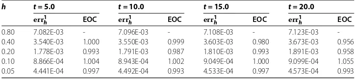
Tables and show computational errors in theL-norm and the energy norm at four
time instancest= .,t= .,t= . andt= ., the corresponding EOC during all
Table 1 Single solitary case: Computational errors in theL2-norm and experimental orders of convergence forP1approximation on a consequence of meshes at time instancest(τ= 10–3)
h t= 5.0 t= 10.0 t= 15.0 t= 20.0
err0h EOC err0h EOC err0h EOC err0h EOC
0.80 2.643E-03 - 3.507E-03 - 4.376E-03 - 5.255E-03
-0.40 6.732E-04 1.973 8.762E-04 2.001 1.099E-03 1.993 1.298E-03 2.017 0.20 1.634E-04 2.043 2.232E-04 1.973 2.605E-04 2.077 3.284E-04 1.983 0.10 4.061E-05 2.009 5.763E-05 1.953 6.561E-05 1.989 8.061E-05 2.026 0.05 1.004E-05 2.016 1.355E-05 2.089 1.638E-05 2.002 2.107E-05 1.936
Table 2 Single solitary case: Computational errors in the energy norm and experimental orders of convergence forP1approximation on a consequence of meshes at time instancest
(τ= 10–3)
h t= 5.0 t= 10.0 t= 15.0 t= 20.0
err1
h EOC err1h EOC err1h EOC err1h EOC
0.80 7.082E-03 - 7.096E-03 - 7.108E-03 - 7.123E-03
-0.40 3.540E-03 1.000 3.550E-03 0.999 3.603E-03 0.980 3.673E-03 0.956 0.20 1.778E-03 0.993 1.791E-03 0.987 1.810E-03 0.993 1.891E-03 0.958 0.10 8.866E-04 1.004 8.943E-04 1.002 9.049E-04 1.000 9.099E-04 1.055 0.05 4.441E-04 0.997 4.492E-04 0.993 4.533E-04 0.997 4.573E-04 0.993
computations. Since the exact solutionu(t) is sufficiently regular over, it follows from Remark that the theoretical error estimates are of orderO(hp+τ). On the other hand, we observe that the numerical experiment of propagation of a single solitary wave indicates a better behavior of EOC in theL-norm, which is expected to be asymptoticallyO(h)
for piecewise linear (p= ) approximations. These observations also correspond with the finite element approach from [], where the same example was studied.
Further, the results for EOC in the energy norm are in a quite good agreement with derived theoretical estimates; in other words, this technique produces an optimal order of convergenceO(hp). Finally, both estimates in Theorem confirm the well-know attribute of DG schemes from the class of convection-diffusion problems,cf.[] and [].
.. Convergence with respect toτ
Secondly, we verify experimentally the convergence of the method in theL-norm and the
energy norm with respect to time stepτ. In order to restrain the discretization errors with respect toh, we use a fine mesh with , elements with piecewise linear approximation. The computations were carried out with five different time stepsτ, see Table . The computational error is evaluated at final timet=Tin theL-norm and the energy norm,
respectively. We observe that both computational errors have EOC of orderO(τ) in the corresponding norms, which is again in a good agreement with derived theoretical results.
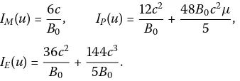
.. Invariant conservation quantities
Similarly as in [], we shall monitor the three conservation quantities for the propagation of the single solitary wave corresponding to mass
IM(u) =
Table 3 Single solitary case: Computational errors in theL2-norm and the energy norm forP1
approximation with respect to time step (h= 0.05)
τ t= 20.0 t= 20.0
err0τ EOC err1τ EOC
0.2000 5.852E-02 - 8.647E-03 -0.1000 2.977E-02 0.975 4.384E-03 1.008 0.0500 1.445E-02 1.046 2.160E-03 0.994 0.0250 7.228E-03 0.996 1.097E-03 0.977 0.0125 3.601E-03 1.005 5.300E-04 1.049
momentum
IP(u) =
u+μudx, ()
and energy
IE(u) =
u+ udx, ()
with respect to the run of the proposed algorithm. The analytical values for the invariants on the entire real domain are given (in []) by
IM(u) = c B
, IP(u) = c
B
+Bc
μ
,
IE(u) = c
B
+c
B
.
()
Moreover, for the purpose of a more accurate comparison with reference results, we introduce the discretel∞-norm defined by
err∞,l≡max k∈J
ul h
x+k––ux+k–,lτ,ulhx–k–ux–k,lτ ()
assessing the accuracy of the method by measuring the difference between the numerical and analytic solutionsuhandu, respectively.
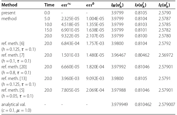
Table records the invariant quantities together with errors err∞, errcomputed on the
finest space-time grid and compares obtained results with several previously presented schemes given in [, , ] and []. All three conservation quantities are kept almost con-stant thus they illustrate the suitability of the proposed scheme for this problem. The ob-tained satisfactory results correspond to the reference ones from [, , ] and []. More-over, we append the recent results from [] in order to compare the incomplete variant of stabilization in dispersion terms with the nonsymmetric one.
5.2 Periodic case
The family of periodic solutions of the RLW equation may be analytically written as (cf.
[])
u(x,t) =A+A·dn
B(x–x–vt),k
Table 4 Single solitary case: Computed invariant quantities and errors in thel∞-norm and theL2-norm (h= 0.05,τ= 10–3)
Method Time err∞ err0 I
M(ulh) IP(ulh) IE(ulh)
present method
0.0 - - 3.9799 0.8105 2.5790
5.0 2.325E-05 1.004E-05 3.9799 0.8104 2.5787 10.0 4.518E-05 1.355E-05 3.9799 0.8103 2.5785 15.0 6.901E-05 1.638E-05 3.9799 0.8101 2.5782 20.0 9.322E-05 2.107E-05 3.9799 0.8100 2.5780
ref. meth. [6] (h= 0.125,τ= 0.1)
20.0 6.843E-04 1.757E-03 3.9800 0.8104 2.5792
ref. meth. [7] (h= 0.1,τ= 0.1)
20.0 1.501E-03 1.480E-05 3.96467 0.80462 2.56972
ref. meth. [20] (h= 0.8,τ= 0.1)
20.0 6.660E-05 1.820E-04 3.97992 0.81046 2.57901
ref. meth. [13] (h= 0.125,τ= 0.1)
20.0 3.960E-03 9.092E-03 3.9800 0.8105 2.5791
ref. meth. [5] (h= 0.05,τ= 0.1)
20.0 7.805E-05 2.069E-04 3.97988 0.81046 2.57901
analytical val. (c= 0.1,μ= 1.0)
- - - 3.979949 0.810462 2.579007
and the parametersA,AandBgiven by
A=c
– –k
√
k–k+
, A=
c
√
k–k+ , ()
B=
εc μ( +εc)
√
k–k+ , ()
wheredn(·,k) is the Jacobi elliptic function andk∈[, ) stands for the elliptic modulus; for definitions and other properties, see []. The exact solution ()-() represents a one-parameter family of periodic waves of amplitudeA+A, traveling with the velocity vin a positivex-direction. The spatial periodωkand time periodTk for each wave are defined by
ωk= K(k)/B and Tk=ωk/v, ()
whereK(k) is a complete elliptic integral of the first kind, see []. The limitk→ implies that the periodic behavior reduces to the propagation of a single solitary wave.
In order to compute the periodic case on approximately the same space-time domain as in the single solitary case, we again set the parameter valuesc= .,x= .,ε=μ= . and the parameterkis experimentally set up ask= . to have periodsTk= . and.
ωk= ...
The run of the algorithm is carried out up to one time periodTkover the problem do-main [–ωk, ωk]. The initial and nonhomogeneous Dirichlet conditions are extracted from the exact solution () and the same linear algebraic solver is used as in the pre-vious case. Figure depicts the propagation of approximation solutions of periodic waves from the initial condition to the final timeTkfor a piecewise linear approximation on the finest considered space-time mesh with time stepτ = . and mesh sizeh= .. Other coarse grids also produce similar plots.
Figure 2 The 3D plot of approximation solutions of periodic waves (left) and corresponding isolines in space-time domain (right).
Table 5 Periodic case: Computational errors in theL2-norm and experimental orders of convergence forP1approximation on a consequence of meshes at time instancest(τ= 10–3)
h t= 5.0 t= 10.0 t= 15.0 t= 20.0
err0
h EOC err0h EOC err0h EOC err0h EOC
0.80 2.790E-02 - 3.589E-02 - 4.531E-02 - 6.290E-02
-0.40 7.016E-03 1.992 9.085E-03 1.982 1.156E-02 1.971 1.612E-03 1.964 0.20 1.860E-03 1.915 2.308E-03 1.977 3.005E-03 1.943 4.281E-03 1.912 0.10 4.952E-04 1.909 6.179E-04 1.901 8.084E-04 1.894 1.204E-04 1.830 0.05 1.357E-04 1.868 1.724E-04 1.841 2.314E-04 1.804 3.534E-04 1.768
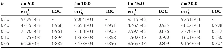
Table 6 Periodic case: Computational errors in the energy norm and experimental orders of convergence forP1approximation on a consequence of meshes at time instancest(τ= 10–3)
h t= 5.0 t= 10.0 t= 15.0 t= 20.0
err1h EOC err1h EOC err1h EOC err1h EOC
0.80 9.029E-03 - 9.004E-03 - 9.115E-03 - 9.251E-03
-0.40 4.615E-03 0.968 4.658E-03 0.951 4.767E-03 0.935 4.862E-03 0.928 0.20 2.370E-03 0.961 2.488E-03 0.905 2.597E-03 0.876 2.770E-03 0.812 0.10 1.275E-03 0.894 1.363E-03 0.868 1.502E-03 0.790 1.601E-03 0.790 0.05 6.906E-04 0.885 7.533E-04 0.856 8.569E-04 0.809 9.154E-04 0.807
.. Convergence with respect to h
Theh-convergence in the periodic case is investigated on a sequence of five successive refined grids partitioning the considered problem domain [–, ]. The choice of time step is again small enough to suppress the influence of time discretization errors, and the computations are performed by piecewise linear approximations, subsequently.
The obtained results recorded in Tables and illustrate the same behavior of com-putational errors in the L-norm and the energy norm with respect to the spatial dis-cretization as in the case of a single solitary wave propagation. The computed EOCs at all four monitoring time instances keep asymptotically the same orders,i.e., err
h=O(h) and err
h=O(h), for piecewise linear approximations and confirm the spatially suboptimal
a priorierror estimates () with respect to theL-norm and spatially optimal estimates
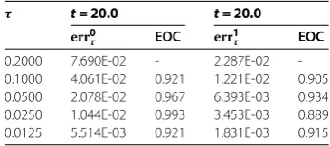
Table 7 Periodic case: Computational errors in theL2-norm and the energy norm forP1
approximation with respect to time step (h= 0.05)
τ t= 20.0 t= 20.0
err0τ EOC err1τ EOC
0.2000 7.690E-02 - 2.287E-02 -0.1000 4.061E-02 0.921 1.221E-02 0.905 0.0500 2.078E-02 0.967 6.393E-03 0.934 0.0250 1.044E-02 0.993 3.453E-03 0.889 0.0125 5.514E-03 0.921 1.831E-03 0.915
Table 8 Periodic case: Computed invariant quantities and errors in thel∞-norm and the
L2-norm (h= 0.05,τ= 10–3)
Method Time err∞ err0 I
M(ulh) IP(ulh) IE(ulh)
present method
0.0 - - 16.5051 3.3180 10.6008
5.0 2.855E-05 1.357E-04 16.5056 3.3180 10.6005 10.0 3.063E-05 1.724E-04 16.5057 3.3179 10.6003 15.0 4.604E-05 2.314E-04 16.5057 3.3178 10.6000 20.0 7.854E-05 3.534E-04 16.5060 3.3178 10.6001
analytical val. (k= 0.63048)
- - - 16.50560 3.318064 10.60086
.. Convergence with respect toτ
The τ-convergence is experimentally verified by the computations on the finest spatial grid having , elements with piecewise linear approximation. The computations are performed by five different time stepsτand monitored at final time of one periodTk. The theoretical results are in accordance with the observations listed in Table ,i.e., err
τ=O(h) and err
τ=O(h).
From the presented numerical results in Sections ..-.. and ..-.., we see that the quality of approximate solutions obtained for a single solitary case and a periodic case is quite comparable.
.. Invariant conservation quantities
Similarly as in Section .., we monitor the preservation of invariants of mass, momen-tum and energy defined by (), () and (), respectively. During the whole period of time, in the course of which the waves propagate inside the periodic domain [–ωk, ωk], all these three invariants of motion remain conserved and equal to their original values that are well-determined analytically att= .
The lack of similar problems in the literature caused that our experiments with peri-odic waves could not be compared with other methods, thus Table captures only the development of errors in thel∞-norm and theL-norm and keeping the invariant
quan-tities during the whole computation performed on the finest space-time grid. All three invariants of motion are not different from their analytical values, according to which this method can be considered suitable also for nonperiodic cases.
6 Conclusion
estimates, namelyO(hp+τ) in theL-norm and in the energy norm. On the other hand,
the presented numerical experiments for single solitary as well as periodic cases signal a better behavior of the experimental (L)-order of convergence, which is expected to be
asymptoticallyO(h+τ) for piecewise linear approximations with a nonsymmetric
vari-ant of interior penalty Galerkin discretizations. In the case of the energy norm, we obtain the optimal experimental order of convergence.
The obtained results confirm that the proposed scheme is a powerful and reliable method for the numerical solution of a nonstationary nonlinear partial differential equa-tion such as the RLW equaequa-tion.
Competing interests
The authors declare that they have no competing interests.
Authors’ contributions
Both authors contributed equally, read and approved the final version of the manuscript.
Author details
1Faculty of Science, Humanities and Education, Technical University of Liberec, Studentská 2, Liberec, 461 17, Czech Republic.2Faculty of Mathematics and Physics, Charles University in Prague, Sokolovská 83, Prague, 186 75, Czech Republic.
Acknowledgements
Dedicated to Professor Hari M Srivastava.
The authors would like to express their sincere gratitude to the referees for valuable comments and helpful suggestions. JH also would like to thank P. ˇCervenková for her assistance with elaboration of numerical experiments. This work was partly supported by the ESF Project No. CZ.1.07/2.3.00/09.0155 ‘Constitution and improvement of a team for demanding technical computations on parallel computers at TU Liberec’ and by SGS Project ‘Modern numerical methods’ financed by TU Liberec.
Received: 14 December 2012 Accepted: 23 April 2013 Published: 7 May 2013
References
1. Peregrine, DH: Calculations of the development of an undular bore. J. Fluid Mech.25, 321-330 (1966)
2. Pava, JA: Nonlinear Dispersive Equations: Existence and Stability of Solitary and Periodic Travelling Wave Solutions. Mathematical Surveys and Monographs, vol. 156. Am. Math. Soc., Providence (2009)
3. Esen, A, Kutluay, S: A finite difference solution of the regularized longwave equation. Math. Probl. Eng.2006, Article ID 85743 (2006)
4. Haq, F, Islam, S, Tirmizi, IA: A numerical technique for solution of the MRLW equation using quarticB-splines. Appl. Math. Model.34(12), 4151-4160 (2010)
5. Islam, S, Haq, S, Ali, A: A meshfree method for the numerical solution of the RLW equation. J. Comput. Appl. Math.
223(2), 997-1012 (2009)
6. Chen, Y, Mei, L: Explicit multistep method for the numerical solution of RLW equation. Appl. Math. Comput.218, 9547-9554 (2012)
7. Dag, I, Ozer, MN: Approximation of the RLW equation by the least square cubicB-spline finite element method. Appl. Math. Model.25, 221-231 (2001)
8. Esen, A, Kutluay, S: Application of a lumped Galerkin method to the regularized long wave equation. Appl. Math. Comput.174(2), 833-845 (2006)
9. Cockburn, B: Discontinuous Galerkin methods for convection dominated problems. In: Barth, TJ, Deconinck, H (eds.) High-Order Methods for Computational Physics. Lecture Notes in Computational Science and Engineering, vol. 9, pp. 69-224. Springer, Berlin (1999)
10. Cockburn, B, Karniadakis, GE, Shu, C-W (eds.): Discontinuous Galerkin Methods. Springer, Berlin (2000)
11. Rivière, B: Discontinuous Galerkin methods for solving elliptic and parabolic equations: theory and implementation. In: Frontiers in Applied Mathematics. SIAM, Philadelphia (2008)
12. Arnold, DN, Brezzi, F, Cockburn, B, Marini, LD: Unified analysis of discontinuous Galerkin methods for elliptic problems. SIAM J. Numer. Anal.39(5), 1749-1779 (2002)
13. Hozman, J: Discontinuous Galerkin method for numerical solution of the regularized long wave equation. AIP Conf. Proc.1497, 118-125 (2012)
14. Dolejší, V, Feistauer, M, Hozman, J: Analysis of semi-implicit DGFEM for nonlinear convection-diffusion problems. Comput. Methods Appl. Mech. Eng.196, 2813-2827 (2007)
15. Dolejší, V, Feistauer, M, Sobotíková, V: Analysis of the discontinuous Galerkin method for nonlinear convection-diffusion problems. Comput. Methods Appl. Mech. Eng.194, 2709-2733 (2005)
16. Feistauer, M, Felcman, J, Straškraba, I: Mathematical and Computational Methods for Compressible Flow. Oxford University Press, Oxford (2003)
18. Ciarlet, PG: The Finite Elements Method for Elliptic Problems. North-Holland, Amsterdam (1979)
19. Kuˇcera, V: Onε-uniform error estimates for singularly perturbed problems in the DG method. In: Numerical Mathematics and Advanced Applications 2011, pp. 368-378 (2013)
20. Djidjeli, K, Price, WG, Twizell, EH, Cao, Q: A linearized implicit pseudo-spectral method for some model equations: the regularized long wave equations. Commun. Numer. Methods Eng.19, 847-863 (2003)
21. Abramowitz, M, Stegun, IA: Handbook of Mathematical Functions. Dover, New York (1965)
doi:10.1186/1687-2770-2013-116