Kernel Mean Shrinkage Estimators
Krikamol Muandet∗ [email protected]
Empirical Inference Department, Max Planck Institute for Intelligent Systems Spemannstraße 38, T¨ubingen 72076, Germany
Bharath Sriperumbudur∗ [email protected]
Department of Statistics, Pennsylvania State University University Park, PA 16802, USA
Kenji Fukumizu [email protected]
The Institute of Statistical Mathematics
10-3 Midoricho, Tachikawa, Tokyo 190-8562 Japan
Arthur Gretton [email protected]
Gatsby Computational Neuroscience Unit, CSML, University College London Alexandra House, 17 Queen Square, London - WC1N 3AR, United Kingdom ORCID 0000-0003-3169-7624
Bernhard Sch¨olkopf [email protected]
Empirical Inference Department, Max Planck Institute for Intelligent Systems Spemannstraße 38, T¨ubingen 72076, Germany
Editor:Ingo Steinwart
Abstract
A mean function in a reproducing kernel Hilbert space (RKHS), or a kernel mean, is central to kernel methods in that it is used by many classical algorithms such as kernel principal component analysis, and it also forms the core inference step of modern kernel methods that rely on embedding probability distributions in RKHSs. Given a finite sample, an empirical average has been used commonly as a standard estimator of the true kernel mean. Despite a widespread use of this estimator, we show that it can be improved thanks to the well-known Stein phenomenon. We propose a new family of estimators called kernel mean shrinkage estimators (KMSEs), which benefit from both theoretical justifications and good empirical performance. The results demonstrate that the proposed estimators outperform
the standard one, especially in a “larged, smalln” paradigm.
Keywords: covariance operator, James-Stein estimators, kernel methods, kernel mean, shrinkage estimators, Stein effect, Tikhonov regularization
1. Introduction
This paper aims to improve the estimation of the mean function in a reproducing kernel Hilbert space (RKHS), or a kernel mean, from a finite sample. A kernel mean is defined with respect to a probability distribution Pover a measurable spaceX by
µP , Z
X
k(x,·) dP(x)∈H, (1)
whereµP is a Bochner integral (see,e.g.,Diestel and Uhl(1977, Chapter 2) andDinculeanu
(2000, Chapter 1) for a definition of Bochner integral) andH is a separable RKHS endowed with a measurable reproducing kernelk:X × X →R such that R
X p
k(x, x) dP(x)<∞.1 Given an i.i.d sample x1, x2, . . . , xn from P, the most natural estimate of the true kernel mean is empirical average
ˆ µP , 1
n
n
X
i=1
k(xi,·). (2)
We refer to this estimator as a kernel mean estimator (KME). Though it is the most commonly used estimator of the true kernel mean, the key contribution of this work is to show that there exist estimators that can improve upon this standard estimator.
The kernel mean has recently gained attention in the machine learning community, thanks to the introduction of Hilbert space embedding for distributions (Berlinet and Thomas-Agnan,2004; Smola et al., 2007). Representing the distribution as a mean func-tion in the RKHS has several advantages. First, if the kernel k is characteristic, the map P7→µP is injective.2 That is, it preserves all information about the distribution (Fukumizu et al.,2004; Sriperumbudur et al.,2008). Second, basic operations on the distribution can be carried out by means of inner products in RKHS,e.g.,EP[f(x)] =hf, µPiHfor allf ∈H,
which is an essential step in probabilistic inference (see, e.g., Song et al.,2011). Lastly, no intermediate density estimation is required, for example, when testing for homogeneity from finite samples. Thus, the algorithms become less susceptible to the curse of dimensionality; see,e.g.,Wasserman (2006, Section 6.5) and Sriperumbudur et al.(2012).
The aforementioned properties make Hilbert space embedding of distributions appealing to many algorithms in modern kernel methods, namely, two-sample testing via maximum mean discrepancy (MMD) (Gretton et al.,2007,2012), kernel independence tests (Gretton et al., 2008), Hilbert space embedding of HMMs (Song et al.,2010), and kernel Bayes rule (Fukumizu et al.,2011). The performance of these algorithms relies directly on the quality of the empirical estimate ˆµP.
In addition, the kernel mean has played much more fundamental role as a basic build-ing block of many kernel-based learnbuild-ing algorithms (Vapnik,1998;Sch¨olkopf et al.,1998). For instance, nonlinear component analyses, such as kernel principal component analysis (KPCA), kernel Fisher discriminant analysis (KFDA), and kernel canonical correlation anal-ysis (KCCA), rely heavily on mean functions and covariance operators in RKHS (Sch¨olkopf et al., 1998;Fukumizu et al.,2007). The kernel K-means algorithm performs clustering in feature space using mean functions as representatives of the clusters (Dhillon et al.,2004). Moreover, the kernel mean also served as a basis in early development of algorithms for clas-sification, density estimation, and anomaly detection (Shawe-Taylor and Cristianini,2004, Chapter 5). All of these employ the empirical average in (2) as an estimate of the true kernel mean.
1. The separability ofHand measurability ofk ensures thatk(·, x) is aH-valued measurable function for
allx∈ X (Steinwart and Christmann,2008, Lemma A.5.18). The separability ofH is guaranteed by
choosingXto be a separable topological space andkto be continuous (Steinwart and Christmann,2008, Lemma 4.33).
We show in this work that the empirical estimator in (2) is, in a certain sense, not opti-mal, i.e., there exist “better” estimators (more below), and then propose simple estimators that outperform the empirical estimator. While it is reasonable to argue that ˆµP is the “best” possible estimator of µP if nothing is known about P (in fact ˆµP is minimax in the
sense ofvan der Vaart (1998, Theorem 25.21, Example 25.24)), in this paper we show that “better” estimators ofµP can be constructed if mild assumptions are made onP. This work is to some extent inspired by Stein’s seminal work in 1955, which showed that the maximum likelihood estimator (MLE) of the mean,θof a multivariate Gaussian distributionN(θ, σ2I) is “inadmissible” (Stein,1955)—i.e., there exists a better estimator—though it is minimax optimal. In particular, Stein showed that there exists an estimator that always achieves smaller total mean squared error regardless of the true θ ∈ Rd, when d≥ 3. Perhaps the best known estimator of such kind is James-Steins estimator (James and Stein,1961). For-mally, if X∼ N(θ, σ2I) withd≥3, the estimator δ(X) =X forθ is inadmissible in mean squared sense and is dominated by the following estimator
δJS(X) =
1−(d−2)σ
2
kXk2
X, (3)
i.e., EkδJS(X)−θk2 ≤ Ekδ(X)−θk2 for all θ and there exists at least one θ for which EkδJS(X)−θk2<Ekδ(X)−θk2.
Interestingly, the James-Stein estimator is itself inadmissible, and there exists a wide class of estimators that outperform the MLE, see, e.g., Berger (1976). Ultimately, Stein’s result suggests that one can construct estimators better than the usual empirical estimator if the relevant parameters are estimated jointly and if the definition of risk ultimately looks at all of these parameters (or coordinates) together. This finding is quite remarkable as it is counter-intuitive as to why joint estimation should yield better estimators when all parameters are mutually independent (Efron and Morris, 1977). Although the Stein phenomenon has been extensively studied in the statistics community, it has not received much attention in the machine learning community.
The James-Stein estimator is a special case of a larger class of estimators known as
shrinkage estimators (Gruber,1998). In its most general form, the shrinkage estimator is a combination of a model with low bias and high variance, and a model with high bias but low variance. For example, one might consider the following estimator:
ˆ
θshrink ,λθ˜+ (1−λ)ˆθML,
For example, if we use the Gaussian RBF kernel (see (6)), the mean functionµP lives in an infinite-dimensional space. As a result, higher moments of the distribution come into play and therefore one cannot adopt Stein’s setting straightforwardly as it involves only the first moment. A direct generalization of James-Stein estimator to infinite-dimensional Hilbert space has been considered, for example, in Berger and Wolpert (1983); Mandelbaum and Shepp(1987);Privault and Rveillac(2008). In those works, the parameter to be estimated is assumed to be the mean of a Gaussian measure on the Hilbert space from which samples are drawn. In contrast, our setting involves samples that are drawn from P defined on an arbitrary measurable space, and not from a Gaussian measure defined on a Hilbert space.
1.1 Contributions
In the following, we present the main contributions of this work.
1. In Section2.2, we propose kernel mean shrinkage estimators and show that these esti-mators can theoretically improve upon the standard empirical estimator, ˆµP in terms of the mean squared error (see Theorem1and Proposition 4), however, requiring the knowledge of the true kernel mean. We relax this condition in Section2.3(see Theo-rem 5) where without requiring the knowledge of the true kernel mean, we construct shrinkage estimators that areuniformly better (in mean squared error) than the em-pirical estimator over a class of distributions P. For bounded continuous translation invariant kernels, we show thatPreduces to a class of distributions whose characteris-tic functions have anL2-norm bounded by a given constant. Through concrete choices forPin Examples 1and 2, we discuss the implications of the proposed estimator.
2. While the proposed estimators in Section2.2and2.3are theoretically interesting, they are not useful in practice as they require the knowledge of the true data generating distribution. In Section2.4(see Theorem7), we present a completely data-dependent estimator (say ˇµP)—referred to as B-KMSE—that is √n-consistent and satisfies
EkµˇP−µPk
2
H<EkµˆP−µPk
2
H+O(n−3/2) as n→ ∞. (4)
3. In Section 3, we present a regularization interpretation for the proposed shrinkage estimator, wherein the shrinkage parameter is shown to be directly related to the regularization parameter. Based on this relation, we present an alternative approach to choosing the shrinkage parameter (different from the one proposed in Section 2.4) through leave-one-out cross-validation, and show that the corresponding shrinkage estimator (we refer to it as R-KMSE) is also√n-consistent and satisfies (4).
to whether S-KMSE with a data-dependent shrinkage parameter is consistent and satisfies an inequality similar to (4). The difficulty in answering these questions lies with the complex form of the estimator, ˜µP which is constructed so as to capture the spectral information of the covariance operator.
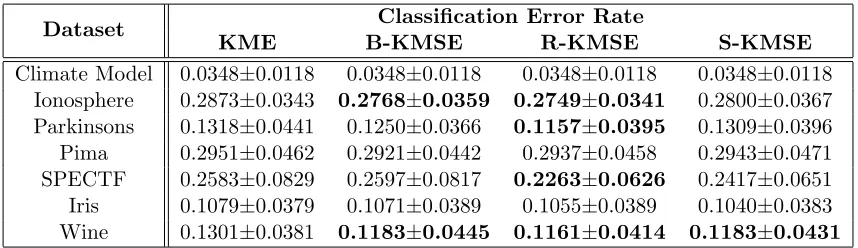
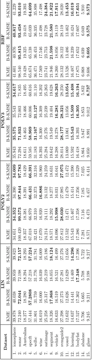
5. In Section6, we empirically evaluate the proposed shrinkage estimators of kernel mean on both synthetic data and several real-world scenarios including Parzen window classification, density estimation and discriminative learning on distributions. The experimental results demonstrate the benefits of our shrinkage estimators over the standard one.
While a shorter version of this work already appeared in Muandet et al. (2014a,b)— particularly, the ideas in Sections2.2,3 and4—, this extended version provides a rigorous theoretical treatment (through Theorems 5, 7, 10, 13 and Proposition 15 which are new) for the proposed estimators and also contains additional experimental results.
2. Kernel Mean Shrinkage Estimators
In this section, we first provide some definitions and notation that are used throughout the paper, following which we present a shrinkage estimator ofµP. The rest of the section presents various properties including the inadmissibility of the empirical estimator.
2.1 Definitions & Notation
For a , (a1, . . . , ad) ∈ Rd, kak2 , q
Pd
i=1a2i. For a topological space X, C(X) (resp.
Cb(X)) denotes the space of all continuous (resp. bounded continuous) functions onX. For
a locally compact Hausdorff space X, f ∈ C(X) is said to vanish at infinity if for every >0 the set {x:|f(x)| ≥} is compact. The class of all continuousf on X which vanish at infinity is denoted as C0(X). Mb(X) (resp. M+1(X)) denotes the set of all finite Borel (resp. probability) measures defined onX. ForX ⊂Rd,Lr(X) denotes the Banach space of
r-power (r≥1) Lebesgue integrable functions. For f ∈Lr(X),kfkLr , R
X|f(x)|rdx 1/r
denotes theLr-norm off for 1≤r <∞. The Fourier transform off ∈L1(Rd) is defined as f∧(ω),(2π)−d/2R
Rdf(x)e
−√−1ω>xdx, ω∈
Rd. The characteristic function ofP∈M+1(Rd) is defined as φP(ω),R
e √
−1ω>xd
P(x), ω∈Rd.
An RKHS over a set X is a Hilbert spaceH consisting of functions onX such that for each x∈ X there is a functionkx ∈H with the property
hf, kxiH=f(x), ∀f ∈H. (5)
The function kx(·) , k(x,·) is called the reproducing kernel of H and the equality (5) is
called the reproducing property of H. The space H is endowed with inner product h·,·iH
and normk · kH. Any symmetric and positive semi-definite kernel functionk:X × X →R
uniquely determines an RKHS (Aronszajn,1950). One of the most popular kernel functions is the Gaussian radial basis function (RBF) kernel onX =Rd,
k(x, y) = exp
−kx−yk
2 2 2σ2
where k · k2 denotes the Euclidean norm and σ > 0 is the bandwidth. For x ∈ H1 and y∈H2,x⊗y denotes the tensor product of x andy, and can be seen as an operator from H2 toH1 as (x⊗y)z=xhy, ziH2 for any z∈H2, whereH1 and H2 are Hilbert spaces.
We assume throughout the paper that we observe a sample x1, x2, . . . , xn ∈ X of size
n drawn independently and identically (i.i.d.) from some unknown distribution P defined over a separable topological spaceX. Denote by µand ˆµ the true kernel mean (1) and its empirical estimate (2) respectively. We remove the subscript for ease of notation, but we will useµP(resp. ˆµP) andµ(resp. ˆµ) interchangeably. For the well-definedness ofµas a Bochner integral, throughout the paper we assume that k is continuous and RXk(x, x) dP(x) < ∞ (see Footnote 1). We measure the quality of an estimator ˜µ∈H of µby the risk function, R:H×H →R,R(µ,µ˜) =Ekµ−µ˜k2H, whereEdenotes the expectation over the choice of random sample of size ndrawn i.i.d. from the distributionP. When ˜µ= ˆµ, for the ease of notation, we will use ∆ to denoteR(µ,µˆ), which can be rewritten as
∆ =Ekµˆ−µk2H=Ekµˆk2H− kµk2H= 1 n2
n
X
i,j=1
Exi,xjk(xi, xj)− kµk
2
H
= 1 n2
n
X
i=1
Exik(xi, xi) +
1 n2
n
X
i6=j
Exi,xjk(xi, xj)− kµk
2
H
= 1
n(Exk(x, x)−Ex,˜xk(x,x˜)), (7) where kµk2
H =Ex,x˜[k(x,x˜)], Ex∼P[Ex˜∼P[k(x,x˜)]] with x and ˜x being independent copies.
An estimator ˆµ1 is said to be as good as µˆ2 ifR(µ,µˆ1) ≤R(µ,µˆ2) for any P, and isbetter
than µˆ2 if it is as good as ˆµ2 and R(µ,µˆ1) < R(µ,µˆ2) for at least one P. An estimator is said to beinadmissible if there exists a better estimator.
2.2 Shrinkage Estimation of µP
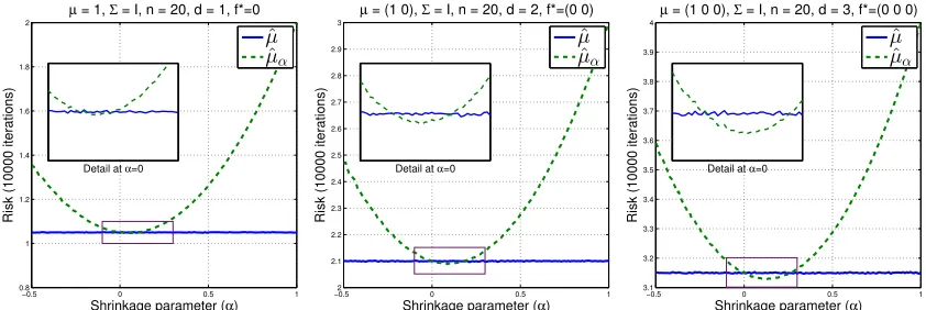
We propose the following kernel mean estimator
ˆ
µα ,αf∗+ (1−α)ˆµ (8)
where α ≥ 0 and f∗ is a fixed, but arbitrary function in H. Basically, it is a shrinkage estimator that shrinks the empirical estimator toward a functionf∗by an amount specified by α. The choice of f∗ can be arbitrary, but we will assume that f∗ is chosen independent of the sample. Ifα= 0, the estimator ˆµα reduces to the empirical estimator ˆµ. We denote
by ∆α the risk of the shrinkage estimator in (8),i.e., ∆α,R(µ,µˆα).
Our first theorem asserts that the shrinkage estimator ˆµαachieves smaller risk than that
of the empirical estimator ˆµgiven an appropriate choice ofα, regardless of the function f∗.
Theorem 1 Let X be a separable topological space. Then for all distributions P and
con-tinuous kernel k satisfyingR k(x, x) dP(x)<∞, ∆α <∆if and only if
α∈
0, 2∆ ∆ +kf∗−µk2
H
. (9)
In particular, arg minα∈R(∆α−∆) is unique and is given by α∗ , ∆+kf∆∗−µk2
Proof Note that
∆α=Ekµˆα−µk2H=kE[ˆµα]−µk2H+Ekµˆα−Eµˆαk2H=kBias(ˆµα)k2H+ Var(ˆµα),
where
Bias(ˆµα) =E[ˆµα]−µ=E[αf∗+ (1−α)ˆµ]−µ=α(f∗−µ)
and
Var(ˆµα) = (1−α)2Ekµˆ−µk2H= (1−α)2∆. Therefore,
∆α=α2kf∗−µk2H+ (1−α)2∆, (10)
i.e., ∆α−∆ =α2
∆ +kf∗−µk2
H−2α∆. This is clearly negative if and only if (9) holds
and is uniquely minimized at α∗ , ∆+kf∆∗−µk2
H.
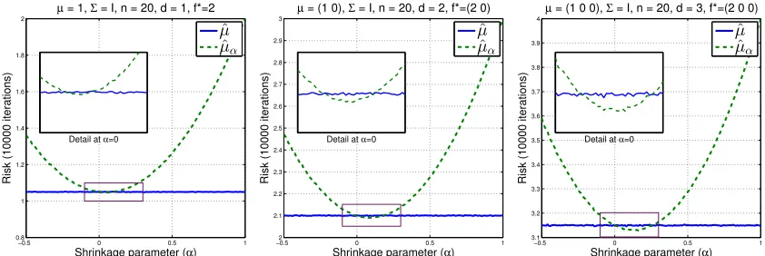
Remark 2 (i) The shrinkage estimator always improves upon the standard one regard-less of the direction of shrinkage, as specified by the choice of f∗. In other words, there exists a wide class of kernel mean estimators that achieve smaller risk than the standard one.
(ii) The range of α depends on the choice of f∗. The further f∗ is from µ, the smaller the range of α becomes. Thus, the shrinkage gets smaller if f∗ is chosen such that it is far from the true kernel mean. This effect is akin to James-Stein estimator.
(iii) From (9), since 0< α <2, i.e., 0<(1−α)2 <1, it follows that Var(ˆµα)<Var(ˆµ) =
∆,i.e., the shrinkage estimator always improves upon the empirical estimator in terms of the variance. Further improvement can be gained by reducing the bias by incorpo-rating the prior knowledge about the location of µ via f∗. This implies that we can potentially gain “twice” by adopting the shrinkage estimator: by reducing variance of the estimator and by incorporating prior knowledge in choosingf∗ such that it is close to the true kernel mean.
While Theorem 1 shows ˆµ to be inadmissible by providing a family of estimators that are better than ˆµ, the result is not useful as all these estimators require the knowledge of µ (which is the parameter of interest) through the range of α given in (9). In Section 2.3, we investigate Theorem 1and show that ˆµα can be constructed under some weak
assump-tions on P, without requiring the knowledge of µ. From (9), the existence of positive α is guaranteed if and only if the risk of the empirical estimator is non-zero. Under some assumptions onk, the following result shows that ∆ = 0 if and only if the distribution Pis a Dirac distribution, i.e., the distribution P is a point mass. This result ensures, in many non-trivial cases, a non-empty range of α for which ∆α−∆<0.
Proposition 3 Let k(x, y) = ψ(x−y), x, y ∈ Rd be a characteristic kernel where ψ ∈ Cb(Rd) is positive definite. Then ∆ = 0if and only if P=δx for some x∈Rd.
2.2.1 Positive-part Shrinkage Estimator
Similar to James-Stein estimator, we can show that the positive-part version of ˆµα also
outperforms ˆµ, where the positive-part estimator is defined by
ˆ
µ+α ,αf∗+ (1−α)+µˆ (11)
with (a)+,aifa >0 and zero otherwise. Equation (11) can be rewritten as
ˆ µ+α =
(
αf∗+ (1−α)ˆµ, 0≤α≤1
αf∗ 1< α <2. (12)
Let ∆+α ,Ekµˆ+α−µk2H be the risk of the positive-part estimator. Then, the following result
shows that ∆+α ≤∆α, given thatα satisfies (9).
Proposition 4 For any α satisfying (9), we have that ∆+α ≤∆α<∆.
Proof According to (12), we decompose the proof into two parts. First, if 0≤α≤1, ˆµα
and ˆµ+α behave exactly the same. Thus, ∆+α = ∆α. On the other hand, when 1 < α <2,
the bias-variance decomposition of these estimators yields
∆α=α2kf∗−µk2H+ (1−α)2Ekµˆ−µk2H and ∆+α =α2kf
∗− µk2H. It is easy to see that ∆+α <∆α when 1< α <2. This concludes the proof.
Proposition 4 implies that, when estimating α, it is better to restrict the value of α to be smaller than 1, although it can be greater than 1, as suggested by Theorem1. The reason is that if 0 ≤ α ≤ 1, the bias is an increasing function of α, whereas the variance is a decreasing function of α. On the other hand, if α > 1, both bias and variance become increasing functions of α. We will see later in Section3 that ˆµα and ˆµ+α can be obtained
naturally as a solution to a regularized regression problem.
2.3 Consequences of Theorem 1
As mentioned before, while Theorem 1 is interesting from the perspective of showing that the shrinkage estimator, ˆµαperforms better—in the mean squared sense—than the empirical
estimator, it unfortunately relies on the fact thatµP (i.e., the object of interest) is known, which makes ˆµα uninteresting. Instead of knowing µP, which requires the knowledge ofP,
in this section, we show that a shrinkage estimator can be constructed that performs better than the empirical estimator, uniformly over a class of probability distributions. To this end, we introduce the notion of an oracle upper bound.
Let P be a class of probability distributions P defined on a measurable space X. We define an oracle upper bound as
Uk,P, inf
P∈P
2∆ ∆ +kf∗−µk2
H
.
It follows immediately from Theorem 1 and the definition of Uk,P that if Uk,P 6= 0, then
of Proposition 3, the class Pcannot contain the Dirac measure δx (for any x ∈Rd) if the kernelkis translation invariant and characteristic onRd. Below we give concrete examples of P for which Uk,P 6= 0 so that the above uniformity statement holds. In particular, we
show in Theorem 5 below that for X =Rd, if a non-trivial bound on the L2-norm of the characteristic function of P is known, it is possible to construct shrinkage estimators that are better (in mean squared error) than the empirical average. In such a case, unlike in Theorem1,αdoes not depend on the individual distributionP, but only on an upper bound associated with a classP.
Theorem 5 Letk(x, y) =ψ(x−y), x, y∈Rd withψ∈C
b(Rd)∩L1(Rd)andψ is a positive
definite function with ψ(0)>0. For a given constant A∈(0,1), let Aψ := A(2π)
d/2ψ(0) kψkL1 and
Pk,A,
n
P∈M+1(Rd) :kφPkL2 ≤
p Aψ
o ,
where φP denotes the characteristic function ofP. Then for all P∈Pk,A,∆α <∆if
α∈
0,
2(1−A)
1 + (n−1)A+nkf∗k2H
ψ(0) +
2n√Akf∗k H
√
ψ(0)
.
Proof By Theorem 1, we have that
∆α <∆, ∀α∈
0, 2∆ ∆ +kf∗−µk2
H
. (13)
Consider
∆ ∆ +kf∗−µk2
H
= Exk(x, x)−Ex,x˜k(x,x˜)
Exk(x, x)−Ex,x˜k(x,x˜) +nkf∗−µk2H (†)
= 1
−Ex,˜xk(x,x˜)
Exk(x,x)
1 + (n−1)Ex,x˜k(x,˜x)
Exk(x,x) +
nkf∗k2
H
Exk(x,x)−
2nhf∗,µi H
Exk(x,x)
≥ 1−
Ex,x˜k(x,˜x)
Exk(x,x)
1 + (n−1)Ex,x˜k(x,˜x)
Exk(x,x) +
nkf∗k2
H
Exk(x,x)+
2nkf∗k H
√
Ex,˜xk(x,x˜)
Exk(x,x)
, (14)
where the division by Exk(x, x) in (†) is valid since Exk(x, x) = ψ(0) >0. Note that the
numerator in the r.h.s. of (14) is non-negative since
Ex,x˜k(x,x˜)≤Ex
p
k(x, x)Ex˜ p
k(˜x,x˜)≤Exk(x, x)
with equality holding if and only ifP=δyfor somey∈Rd(see Proposition3). However, for any A∈(0,1) and y∈Rd, it is easy to verify thatδ
y ∈/ Pk,A, which implies the numerator
in fact positive. The denominator is clearly positive sinceEx,x˜k(x,x˜)≥0 and therefore the r.h.s. of (14) is positive. Also note that
Ex,˜xk(x,x˜) =
Z Z
ψ(x−y) dP(x) dP(y) (∗) =
Z
≤ sup
ω∈Rd
ψ∧(ω)kφPk2
L2 ≤(2π)
−d/2kψk
L1kφPk
2
L2, (15)
whereψ∧is the Fourier transform ofψand (∗) follows—see (16) in the proof of Proposition 5 inSriperumbudur et al.(2011)—by invoking Bochner’s theorem (Wendland,2005, Theorem 6.6), which states that ψ is Fourier transform of a non-negative finite Borel measure with density (2π)−d/2ψ∧,i.e.,ψ(x) = (2π)−d/2R e−ix>ωψ∧(ω) dω,x∈Rd. AsExk(x, x) =ψ(0),
we have that
Ex,x˜k(x,x˜) Exk(x, x)
≤ AkφPk
2
L2
Aψ
and therefore for any P ∈ Pk,A, Ex,˜x k(x,x˜)
Exk(x,x) ≤ A. Using this in (14) and combining it with
(13) yields the result.
Remark 6 (i) Theorem 5 shows that for any P ∈ Pk,A, it is possible to construct a
shrinkage estimator that dominates the empirical estimator, i.e., the shrinkage esti-mator has a strictly smaller risk than that of the empirical estiesti-mator.
(ii) Suppose that P has a density, denoted by p, with respect to the Lebesgue measure and φP ∈L2(
Rd). By Plancherel’s theorem, p∈L2(Rd) as kpkL2 =kφPkL2, which means that Pk,A includes distributions with square integrable densities (note that in general
not every p is square integrable). Since
kφPk2L2 = Z
|φP(ω)|2 dω≤ sup
ω∈Rd
|φP(ω)|
Z
|φP(ω)|dω=kφPkL1,
where we used the fact that supω∈Rd|φP(ω)|= 1, it is easy to check that
(
P∈M+1(Rd) :kφPkL1 ≤
A(2π)d/2ψ(0)
kψkL1
)
⊂Pk,A.
This means bounded densities belong to Pk,A as φP ∈ L1(Rd) implies that P has a density, p∈C0(Rd). Moreover, it is easy to check that larger the value ofA, larger is
the classPk,A and smaller is the range of α for which ∆α <∆and vice-versa.
In the following, we present some concrete examples to elucidate Theorem 5.
Example 1 (Gaussian kernel and Gaussian distribution) Define
N,
P∈M+1(Rd)
dP(x) = 1 (2πσ2)d/2e
−kx−θk22
2σ2 dx, θ∈Rd, σ >0
,
where ψ(x) =e−kxk22/2τ2, x∈Rd and τ >0. For P∈N, it is easy to verify that φP(ω) =e
√
−1θ>ω−1 2σ
2kωk2
2, ω ∈Rd and kφ
Pk
2
L2 =
Z
Example 2 (Linear kernel) Suppose f∗ = 0 and k(x, y) = x>y. While the setting of Theorem 5 does not fit this choice of k, an inspection of its proof shows that it is possible to construct a shrinkage estimator that improves upon µP for an appropriate class of dis-tributions. To this end, let ϑ and Σ represent the mean vector and covariance matrix of a distribution P defined on Rd. Then it is easy to check that EEx,xx˜kk((x,xx,x˜)) = kϑk
2 2
trace(Σ)+kϑk2 2
and therefore for a given A∈(0,1), define
Pk,A,
P∈M+1(Rd)
kϑk2 2 trace(Σ) ≤
A 1−A
.
From (13) and (14), it is clear that for anyP∈Pk,A, ∆α <∆ if α∈
0,1+(2(1n−−A1))Ai. Note that this choice of kernel yields the setting similar to classical James-Stein estimation. In James-Stein estimation, P∈N (see Example 1 for the definition of N) and ϑis estimated
as (1−α˜) ˆϑ—which improves upon ϑˆ—whereα˜ depends on the sample (xi)ni=1 and ϑˆis the
sample mean. In our case, for all P ∈ Pk,A =
n
P∈N : kϑk2 ≤σ q
dA
1−A
o
, ∆α < ∆ if
α ∈ 0,1+(2(1n−−A1))Ai. In addition, in contrast to the James-stein estimator which improves upon the empirical estimator (i.e., sample mean) for only d ≥ 3, we note here that the proposed estimator improves for anydas long as P∈Pk,A. On the other hand, the proposed
estimator requires some knowledge about the distribution (particularly a bound on kϑk2), which the James-Stein estimator does not (see Section2.5 for more details).
2.4 Data-Dependent Shrinkage Parameter
The discussion so far showed that the shrinkage estimator in (8) performs better than the empirical estimator if the data generating distribution satisfies a certain mild condition (see Theorem 5; Examples 1 and 2). However, since this condition is usually not checkable in practice, the shrinkage estimator lacks applicability. In this section, we present a completely data driven shrinkage estimator by estimating the shrinkage parameterαfrom data so that the estimator does not require any knowledge of the data generating distribution.
Since the maximal difference between ∆α and ∆ occurs at α∗ (see Theorem 1), given
an i.i.d. sampleX={x1, x2, . . . , xn}fromP, we propose to estimateµusing ˆµα˜ = (1−α˜)ˆµ (i.e., assumingf∗= 0) where ˜α is an estimator of α∗ = ∆/(∆ +kµk2
H) given by
˜
α= ∆ˆ ˆ
∆ +kµˆk2
H
, (16)
with ˆ∆ and ˆµ being the empirical versions of ∆ and µ, respectively (see Theorem 7 for precise definitions). The following result shows that ˜α is a n√n-consistent estimator ofα∗ and kµˆα˜−µkH concentrates aroundkµˆα∗−µkH. In addition, we show that
∆α∗≤∆α˜ ≤∆α∗+O(n
−3/2) as n→ ∞,
which means the performance of ˆµα˜ is similar to that of the best estimator (in mean squared sense) of the form ˆµα. In what follows, we will call the estimator ˆµα˜ an empirical-bound
Theorem 7 Suppose n ≥ 2 and f∗ = 0. Let k be a continuous kernel on a separable topological space X satisfyingRXk(x, x) dP(x)<∞. Define
ˆ ∆,
ˆ
Ek(x, x)−Ekˆ (x,x˜)
n and kµˆk
2
H, n12
n
X
i,j=1
k(xi, xj)
where Eˆk(x, x) , n1
Pn
i=1k(xi, xi) and Eˆk(x,x˜) ,
1
n(n−1)
Pn
i6=jk(xi, xj) are the empirical
estimators of Exk(x, x) and Ex,x˜k(x,x˜) respectively. Assume there exist finite constants κ1 >0,κ2>0, σ1 >0 and σ2 >0 such that
Ekk(·, x)−µkmH ≤ m! 2 σ
2
1κm1−2, ∀m≥2. (17)
and
E|k(x, x)−Exk(x, x)|m ≤
m! 2 σ
2 2κm
−2
2 , ∀m≥2. (18)
Then
|α˜−α∗|=OP(n−3/2) and
kµˆα˜ −µkH− kµˆα∗−µkH
=OP(n −3/2)
as n→ ∞. In particular,
min
α Ekµˆα−µk
2
H≤Ekµˆα˜ −µk2H≤min
α Ekµˆα−µk
2
H+O(n−3/2) (19)
as n→ ∞.
Proof See Section 5.2.
Remark 8 (i) µˆα˜ is a
√
n-consistent estimator of µ. This follows from
kµˆα˜−µkH≤ kµˆα∗−µkH+OP(n
−3/2)
≤(1−α∗)kµˆ−µkH+α∗kµkH+OP(n−3/2)
with
α∗= ∆
∆ +kµk2
H
= Exk(x, x)−Ex,˜xk(x,x˜) Exk(x, x) + (n−1)Ex,x˜k(x,x˜)
=O(n−1)
as n→ ∞. Using (38), we obtain kµˆα˜−µkH=OP(n
−1/2) as n→ ∞, which implies
thatµˆα˜ is a
√
n-consistent estimator of µ.
(ii) Equation (19) shows that∆˜α ≤∆α∗+O(n
−3/2) where ∆
α∗<∆(see Theorem 1) and therefore for any P satisfying (17) and (18), ∆˜α <∆ +O(n−3/2) as n→ ∞.
(iii) Suppose the kernel is bounded, i.e., supx,y∈X|k(x, y)| ≤ κ < ∞. Then it is easy to
verify that (17) and (18) hold with σ1 =
√
κ, κ1 = 2
√
κ, σ2 = κ and κ2 = 2κ and
therefore the claims in Theorem 7 hold for bounded kernels.
(iv) Fork(x, y) =x>y, we have
Ekk(·, x)−µkmH =E kk(·, x)−µk2Hm/2 =E kx−Exxk22 m/2
and
E|k(x, x)−Exk(x, x)|m =E|kxk22−Exkxk22|m.
The conditions in (17) and (18) hold for P ∈ N where N is defined in Example 1.
With P∈N and k(x, y) =x>y, the problem of estimating µ reduces to estimating θ,
for which we have presented a James-Stein-like estimator, µˆα˜ that satisfies the oracle
inequality in (19).
(v) While the moment conditions in (17) and (18) are obviously satisfied by bounded kernels, for unbounded kernels, these conditions are quite stringent as they require all the higher moments to exist. These conditions can be weakened and the proof of Theorem 7 can be carried out using Chebyshev inequality instead of Bernstein’s inequality but at the cost of a slow rate in (19).
2.5 Connection to James-Stein Estimator
In this section, we explore the connection of our proposed estimator in (8) to the James-Stein estimator. Recall that James-Stein’s setting deals with estimating the mean of the Gaussian distribution N(θ, σ2I
d), which can be viewed as a special case of kernel mean estimation
when we restrict to the class of distributionsP,{N(θ, σ2Id)|θ∈Rd} and a linear kernel k(x, y) =x>y, x, y ∈Rd (see Example 2). In this case, it is easy to verify that ∆ =dσ2/n and ∆α <∆ for
α∈
0, 2dσ 2 dσ2+nkθk2
.
Let us assume that n = 1, in which case, we obtain ∆α < ∆ for α ∈
0, 2dσ2
Exkxk2
as
Exkxk2 =kθk2+dσ2. Note that the choice ofα is dependent on P through Exkxk2 which
is not known in practice. To this end, we replace it with the empirical version kxk2 that depends only on the samplex. For an arbitrary constantc∈(0,2d), the shrinkage estimator (assumingf∗ = 0) can thus be written as
ˆ
µα = (1−α)ˆµ=
1− cσ
2
kxk2
x=x−cσ
2x
kxk2,
which is exactly the James-Stein estimator in (3). This particular way of estimating the shrinkage parameter α has an intriguing consequence, as shown in Stein’s seminal works (Stein, 1955; James and Stein, 1961), that the shrinkage estimator ˆµα can be shown to
dominate the maximum likelihood estimator ˆµuniformly over all θ.
While it is compelling to see that there is seemingly a fundamental principle underlying both these settings, this connection also reveals crucial difference between our approach and classical setting of Stein—notably, original James-Stein estimator improves upon the sample mean even when α is data-dependent (see ˆµα above), however, with the crucial
assumption thatx is normally distributed.
3. Kernel Mean Estimation as Regression Problem
we provide a regression perspective to shrinkage estimation. The starting point of the connection between regression and shrinkage estimation is the observation that the kernel mean µP and its empirical estimate ˆµP can be obtained as minimizers of the following risk functionals,
E(g), Z
X
kk(·, x)−gk2H dP(x) and Eb(g), 1 n
n
X
i=1
kk(·, xi)−gk2H,
respectively (Kim and Scott, 2012). Given these formulations, it is natural to ask if min-imizing the regularized version ofEb(g) will give a “better” estimator. While this question is interesting, it has to be noted that in principle, there is really no need to consider a regularized formulation as the problem of minimizingEbis not ill-posed, unlike in function estimation or regression problems. To investigate this question, we consider the minimiza-tion of the following regularized empirical risk funcminimiza-tional,
b
Eλ(g),Eb(g) +λΩ(kgkH) = 1 n
n
X
i=1
kk(·, xi)−gkH2 +λΩ(kgkH), (20)
where Ω : R+ → R+ denotes a monotonically increasing function and λ > 0 is the regularization parameter. By representer theorem (Sch¨olkopf et al., 2001), any function g∈H that is a minimizer of (20) lies in a subspace spanned by {k(·, x1), . . . , k(·, xn)},i.e.,
g =Pn
j=1βjk(·, xj) for some β,[β1, . . . , βn] > ∈
Rn. Hence, by setting Ω(kgkH) =kgk2H,
we can rewrite (20) in terms of βas
b
E(g) +λΩ(kgkH) =β>Kβ−2β>K1n+λβ>Kβ+c, (21)
whereK is ann×n Gram matrix such thatKij =k(xi, xj), cis a constant that does not
depend on β, and 1n = [1/n,1/n, . . . ,1/n]>. Differentiating (21) with respect to β and
setting it to zero yields an optimal weight vector β = 1+1λ1n and so the minimizer of
(20) is given by
ˆ µλ=
1 1 +λµˆ=
1− λ
1 +λ
ˆ
µ,(1−α)ˆµ, (22)
which is nothing but the shrinkage estimator in (8) withα= 1+λλ andf∗= 0. This provides a nice relation between shrinkage estimation and regularized risk minimization, wherein the regularization helps in shrinking the estimator ˆµ towards zero although it is not required from the point of view of ill-posedness. In particular, since 0<1−α <1, ˆµλ corresponds
to a positive-part estimator proposed in Section 2.2.1when f∗ = 0.
Note that ˆµλ is a consistent estimator of µasλ→0 andn→ ∞, which follows from
kµˆλ−µkH≤
1
1 +λkµˆ−µkH+ λ
1 +λkµkH≤OP(n
−1/2) +O(λ).
In particular λ = τ n−1/2 (for some constant τ > 0) yields the slowest possible rate for λ→ 0 such that the best possible rate ofn−1/2 is obtained forkµˆλ−µkH →0 as n→ ∞.
τ ∈0, 2 √
n∆
kµk2
H−∆
. Note that ˆµλ is not useful in practice asλis not knowna priori. However,
by choosing
λ= ∆ˆ
kµˆk2
H
,
it is easy to verify (see Theorem7 and Remark8) that
Ekµˆλ−µk2H<Ekµˆ−µk2H+O(n−3/2) (23) as n → ∞. Owing to the connection of ˆµλ to a regression problem, in the following, we
present an alternate data-dependent choice ofλobtained from leave-one-out cross validation (LOOCV) that also satisfies (23), and we refer to the corresponding estimator asregularized kernel mean shrinkage estimator (R-KMSE).
To this end, for a given shrinkage parameter λ, denote by ˆµ(λ−i)as the kernel mean esti-mated from{xj}nj=1\{xi}. We will measure the quality of ˆµ(
−i)
λ by how well it approximates
k(·, xi) with the overall quality being quantified by the cross-validation score,
LOOCV(λ) = 1 n
n
X
i=1
k(·, xi)−µˆ (−i)
λ
2
H. (24)
The LOOCV formulation in (24) differs from the one used in regression, wherein instead of measuring the deviation of the prediction made by the function on the omitted observation, we measure the deviation between the feature map of the omitted observation and the function itself. The following result shows that the shrinkage parameter in ˆµλ (see (22))
can be obtained analytically by minimizing (24) and requiresO(n2) operations to compute. Proposition 9 Let n ≥ 2, ρ := n12
Pn
i,j=1k(xi, xj) and % := n1 Pni=1k(xi, xi). Assuming
nρ > %, the unique minimizer of LOOCV(λ) is given by
λr =
n(%−ρ)
(n−1)(nρ−%). (25)
Proof See Section 5.3.
It is instructive to compare
αr =
λr
λr+ 1
= %−ρ
(n−2)ρ+%/n (26)
to the one in (16), where the latter can be shown to be %+(%n−−ρ2)ρ, by noting that ˆEk(x, x) =% and ˆEk(x,x˜) = nρn−−1% (in Theorem 7, we employ the U-statistic estimator of Ex,x˜k(x,x˜), whereas ρ in Proposition 9 can be seen as a V-statistic counterpart). This means αr
obtained from LOOCV will be relatively larger than the one obtained from (16). Like in Theorem 7, the requirement that n ≥ 2 in Theorem 9 stems from the fact that at least two data points are needed to evaluate the LOOCV score. Note that nρ > % if and only if ˆEk(x,x˜) > 0, which is guaranteed if the kernel is positive valued. We refer to ˆµλr as
Theorem 10 Let n≥2,nρ > %where ρ and% are defined in Proposition 9 andksatisfies the assumptions in Theorem 7. Then kµˆλr −µkH=OP(n
−1/2), min
α Ekµˆα−µk
2
H≤Ekµˆλr−µk
2
H≤minα Ekµˆα−µk2H+O(n−3/2) (27)
where µˆα = (1−α)ˆµ and therefore
Ekµˆλr −µk
2
H<Ekµˆ−µkH2 +O(n−3/2) (28)
as n→ ∞.
Proof See Section 5.4.
4. Spectral Shrinkage Estimators
Consider the following regularized risk minimization problem
arg infF∈H⊗H Ex∼Pkk(x,·)−F[k(x,·)]k2H+λkFk2HS, (29) where the minimization is carried over the space of Hilbert-Schmidt operators,FonHwith
kFkHSbeing the Hilbert-Schmidt norm ofF. As an interpretation, we are finding a smooth operatorFthat mapsk(x,·) to itself (seeGr¨unew¨alder et al.(2013) for more details on this smooth operator framework). It is not difficult to show that the solution to (29) is given by F = ΣXX(ΣXX +λI)−1 where ΣXX =
R
k(·.x)⊗k(·, x) dP(x) is a covariance operator defined on H (see, e.g., Gr¨unew¨alder et al., 2012). Note that ΣXX is a Bochner integral,
which is well-defined as a Hilbert-Schmidt operator if X is a separable topological space and kis a continuous kernel satisfyingR
k(x, x) dP(x)<∞. Consequently, let us define
µλ=Fµ= ΣXX(ΣXX +λI)−1µ,
which is an approximation to µ as it can be shown that kµλ−µkH→ 0 as λ→0 (see the
proof of Theorem 13). Given an i.i.d. sample x1, . . . , xn from P, the empirical counterpart of (29) is given by
arg minF∈H⊗H 1 n
n
X
i=1
kk(xi,·)−F[k(xi,·)]k2H+λkFk2HS (30)
resulting in
ˇ
µλ ,Fˆµ= ˆΣXX( ˆΣXX +λI)−1µˆ (31)
where ˆΣXX is the empirical covariance operator on H given by
ˆ ΣXX =
1 n
n
X
i=1
k(·.xi)⊗k(·, xi).
Unlike ˆµλ in (22), ˇµλ shrinks ˆµdifferently in each coordinate by taking the eigenspectrum
of ˆΣXX into account (see Proposition11) and so we refer to it as the spectral kernel mean
Proposition 11 Let {(γi, φi)}ni=1 be eigenvalue and eigenfunction pairs of ΣˆXX. Then
ˇ µλ=
n
X
i=1
γi
γi+λ
hµ, φˆ iiHφi.
Proof Since ˆΣXX is a finite rank operator, it is compact. Since it is also a self-adjoint
op-erator onH, by Hilbert-Schmidt theorem (Reed and Simon,1972, Theorems VI.16, VI.17), we have ˆΣXX =
Pn
i=1γihφi,·iHφi. The result follows by using this in (31).
As shown in Proposition 11, the effect of S-KMSE is to reduce the contribution of high frequency components of ˆµ (i.e., contribution of ˆµ along the directions corresponding to smaller γi) when ˆµ is expanded in terms of the eigenfunctions of the empirical covariance
operator, which are nothing but the kernel PCA basis (Rasmussen and Williams, 2006, Section 4.3). This means, similar to R-KMSE, S-KMSE also shrinks ˆµtowards zero, how-ever, the difference being that while R-KMSE shrinks equally in all coordinates, S-KMSE controls the amount of shrinkage by the information contained in each coordinate. In par-ticular, S-KMSE takes into account more information about the kernel by allowing for different amount of shrinkage in each coordinate direction according to the value of γi,
wherein the shrinkage is small in the coordinates whoseγi are large. Moreover, Proposition
11 reveals that the effect of shrinkage is akin to spectral filtering (Bauer et al., 2007)— which in our case corresponds to Tikhonov regularization—wherein S-KMSE filters out the high-frequency components of the spectral representation of the kernel mean. Muandet et al. (2014b) leverages this observation and generalizes S-KMSE to a family of shrinkage estimators via spectral filtering algorithms.
The following result presents an alternate representation for ˇµλ, using which we relate
the smooth operator formulation in (30) to the regularization formulation in (20).
Proposition 12 Let Φ :Rn→H, a7→Pni=1aik(·, xi) where a,(a1, . . . , an). Then
ˇ
µλ= ˆΣXX( ˆΣXX +λI)−1µˆ= Φ(K+nλI)−1K1n,
where K is the Gram matrix,I is an identity operator on H, I is an n×n identity matrix and 1n,[1/n, . . . ,1/n]>.
Proof See Section 5.5.
From Proposition12, it is clear that
ˇ µλ =
1
√
n
n
X
j=1
(βs)jk(·, xj) (32)
whereβs,
√
n(K+nλI)−1K1
n. Given the form of ˇµλ in (32), it is easy to verify that βs
is the minimizer of (20) when Ebλ is minimized over {g = √1
n
Pn
j=1(β)jk(·, xj) : β ∈ Rn}
with Ω(kgkH),kβk2 2.
Theorem 13 Suppose X is a separable topological space and k is a continuous, bounded kernel on X. Then the following hold.
(i) If µ∈ R(ΣXX), then kµˇλ−µkH→0 asλ
√
n→ ∞, λ→0 and n→ ∞.
(ii) If µ ∈ R(ΣXX), then kµˇλ −µkH = OP(n
−1/2) for λ = cn−1/2 with c > 0 being a
constant independent of n.
Proof See Section 5.6.
Remark 14 While Theorem 13(i) shows that S-KMSE, µˇλ is not universally consistent,
i.e., S-KMSE is not consistent for all P but only for those P that satisfies µ ∈ R(ΣXX),
under some additional conditions on the kernel, the universal consistency of S-KMSE can be guaranteed. This is achieved by assuming that constant functions are included in H,
i.e., 1 ∈ H. Note that if 1 ∈ H, then it is easy to check that there exists g ∈ H (choose
g = 1) such that µ = ΣXXg =
R
k(·, x)g(x) dP(x), i.e., µ ∈ R(ΣXX), and, therefore, by
Theorem13,µˇλis not only universally consistent but also achieves a rate ofn−1/2. Choosing
k(x, y) = ˜k(x, y) +b, x, y ∈ X, b > 0 where ˜k is any bounded, continuous positive definite kernel ensures that 1∈H.
Note that the estimator ˇµλ requires the knowledge of the shrinkage or regularization
pa-rameter, λ. Similar to R-KMSE, below, we present a data dependent approach to selectλ using leave-one-out cross validation. While the shrinkage parameter for R-KMSE can be obtained in a simple closed form (see Proposition 9), we will see below that finding the corresponding parameter for S-KMSE is more involved. Evaluating the score function (i.e., (24)) na¨ıvely requires one to solve for ˆµ(λ−i) explicitly for everyi, which is computationally expensive. The following result provides an alternate expression for the score, which can be evaluated efficiently. We would like to point out that a variation of Proposition 15 already appeared in Muandet et al. (2014a, Theorem 4). However, Theorem 4 in Muandet et al.
(2014a) uses an inappropriate choice of ˆµ(λ−i), which we fixed in the following result. Proposition 15 The LOOCV score of S-KMSE is given by
LOOCV(λ) = 1
ntr (K+λnI)
−1K(K+λ
nI)−1Aλ
− 2
ntr (K+λnI) −1B
λ
+1 n
n
X
i=1
k(xi, xi),
where λn , (n−1)λ, Aλ , (n−11)2
Pn
i=1ci,λc>i,λ, Bλ , n−11Pni=1ci,λk>i , di,λ , k>i (K+
λnI)−1ei,
ci,λ ,K1−ki−eiki>1+eik(xi, xi) +
eik>i (K+λnI)−1K1
1−di,λ
−eik
>
i (K+λnI)
−1k
i
1−di,λ
−eik
>
i (K+λnI)−1eik>i 1
1−di,λ
+eik >
i (K+λnI)−1eik(xi, xi)
1−di,λ
,
ki is the ith column of K, 1,(1, . . . ,1)> and ei,(0,0, . . . ,1, . . . ,0)> with 1 being in the
Proof See Section 5.7.
Unlike R-KMSE, a closed form expression for the minimizer ofLOOCV(λ) in Proposition15
is not possible and so proving the consistency of S-KMSE along with results similar to those in Theorem 10 are highly non-trivial. Hence, we are not able to provide any theoretical comparison of ˇµλ(withλbeing chosen as a minimizer ofLOOCV(λ) in Proposition15) with
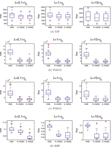
ˆ
µ. However, in the next section, we provide an empirical comparison through simulations where we show that the S-KMSE outperforms the empirical estimator.
5. Proofs
In this section, we present the missing proofs of the results of Sections 2–4.
5.1 Proof of Proposition 3
( ⇒ ) IfP=δx for somex∈ X, then ˆµ=µ=k(·, x) and thus ∆ = 0.
( ⇐) Suppose ∆ = 0. It follows from (7) thatRR
(k(x, x)−k(x, y)) dP(x) dP(y) = 0. Since kis translation invariant, this reduces to
Z Z
(ψ(0)−ψ(x−y)) dP(x) dP(y) = 0.
By invoking Bochner’s theorem (Wendland,2005, Theorem 6.6), which states that ψis the Fourier transform of a non-negative finite Borel measure Λ,i.e.,ψ(x) =Re−ix>ωdΛ(ω), x∈
Rd, we obtain (see (16) in the proof of Proposition 5 in Sriperumbudur et al. (2011))
Z Z
ψ(x−y) dP(x) dP(y) = Z
|φP(ω)|2dΛ(ω), thereby yielding
Z
(|φP(ω)|2−1) dΛ(ω) = 0, (33) where φP is the characteristic function of P. Note that φP is uniformly continuous and |φP| ≤ 1. Since k is characteristic, Theorem 9 inSriperumbudur et al. (2010) implies that supp(Λ) = Rd, using which in (33) yields |φP(ω)| = 1 for allω ∈Rd. Since φP is positive
definite onRd, it follows fromSasv´ari(2013, Lemma 1.5.1) thatφP(ω) =e
√ −1ω>x
for some x∈Rd and thus P=δx.
5.2 Proof of Theorem 7
Before we prove Theorem 7, we present Bernstein’s inequality in separable Hilbert spaces, quoted from Yurinsky(1995, Theorem 3.3.4), which will be used to prove Theorem 7.
Theorem 16 (Bernstein’s inequality) Let (Ω,A, P) be a probability space,H be a sep-arable Hilbert space, B > 0 and θ > 0. Furthermore, let ξ1, . . . , ξn : Ω →H be zero mean
independent random variables satisfying
n
X
i=1
EkξikmH ≤
m! 2 θ
Then for any τ >0,
Pn (
(ξ1, . . . , ξn) :
n
X
i=1
ξi
H
≥2Bτ +
√
2θ2τ )
≤2e−τ.
Proof (of Theorem 7) Consider
˜
α−α∗ = ∆ˆ ˆ
∆ +kµˆk2
H
− ∆
∆ +kµk2
H
= ˆ ∆kµk2
H−∆kµˆk2H
( ˆ∆ +kµˆk2
H)(∆ +kµk2H)
= ˆ ∆(kµk2
H− kµˆk2H)
(∆ +kµk2
H)( ˆ∆ +kµˆk2H)
+ ( ˆ∆−∆)kµˆk 2
H
(∆ +kµk2
H)( ˆ∆ +kµˆk2H)
= α˜(kµk 2
H− kµˆk2H)
(∆ +kµk2
H)
+( ˆ∆−∆)(1−α˜) (∆ +kµk2
H)
.
Rearranging ˜α, we obtain
˜
α−α∗ = α∗(kµk 2
H− kµˆk2H) + (1−α∗)( ˆ∆−∆)
ˆ
∆ +kµˆk2
H
.
Therefore,
|α˜−α∗| ≤ α∗|kµk
2
H− kµˆk2H|+ (1 +α∗)|∆ˆ −∆|
(∆ +kµk2
H)−(kµk2H− kµˆk2H) + ( ˆ∆−∆)
, (35)
where it is easy to verify that
|∆ˆ −∆| ≤ |Ex,˜xk(x,x˜)−Eˆk(x,x˜)|
n +
|Ekˆ (x, x)−Exk(x, x)|
n . (36)
In the following we obtain bounds on |Eˆk(x, x)−Exk(x, x)|, |Ex,x˜k(x,x˜)−Eˆk(x,x˜)| and
|kµk2
H− kµˆk2H|when the kernel satisfies (17) and (18).
Bound on |Eˆk(x, x)−Exk(x, x)|:
Since k is a continuous kernel on a separable topological space X, it follows from Lemma 4.33 ofSteinwart and Christmann (2008) that H is separable. By defining ξi ,k(xi, xi)−
Exk(x.x), it follows from (18) that θ=
√
nσ2 and B =κ2 and so by Theorem 16, for any τ >0, with probability at least 1−2e−τ,
|Eˆk(x, x)−Exk(x, x)| ≤
r 2σ2
2τ
n +
2κ2τ
n . (37)
Bound on kµˆ−µkH:
By defining ξi,k(·, xi)−µand using (17), we haveθ=
√
nσ1 and B =κ1. Therefore, by Theorem16, for anyτ >0, with probability at least 1−2e−τ,
kµˆ−µkH≤
r 2σ12τ
n +
2κ1τ
n . (38)
Bound on |kµˆk2
Since
kµˆk2H− kµk2H
≤(kµˆkH+kµkH)kµˆ−µkH≤(kµˆ−µkH+ 2kµkH)kµˆ−µkH,
it follows from (38) that for any τ >0, with probability at least 1−2e−τ,
kµˆk2H− kµk2H ≤D1
r τ n +D2
τ n
+D3
τ n
3/2 +D4
τ n
2
, (39)
where (Di)4i=1 are positive constants that depend only on σ12, κ and kµkH, and not on n and τ.
Bound on |Eˆk(x,x˜)−Ex,x˜k(x,x˜)|: Since
ˆ
Ek(x,x˜)−Ex,x˜k(x,x˜) =
n2(kµˆk2
H− kµk2H) +n(Exk(x, x)−Eˆk(x, x)) +n(kµk2H−Exk(x, x))
n(n−1) ,
it follows from (37) and (39) that for anyτ >0, with probability at least 1−4e−τ,
|Eˆk(x,x˜)−Ex,x˜k(x,x˜)| ≤F1 r
τ n+F2
τ n
+F3
τ n
3/2 +F4
τ n
2 +F5
n
≤F10 r
1 +τ n +F
0 2
1 +τ
n
+F30
1 +τ n
3/2 +F40
1 +τ
n 2
, (40)
where (Fi)5i=1 and (Fi0)4i=1 are positive constants that do not depend onnand τ. Bound on |α˜−α∗|:
Using (37) and (40) in (36), for anyτ >0, with probability at least 1−4e−τ,
|∆ˆ −∆| ≤ F
00 1 n
r 1 +τ
n +
F200 n
1 +τ
n + F 00 3 n 1 +τ
n 3/2
+F 00 4 n
1 +τ
n 2
,
using which in (35) along with (39), we obtain that for anyτ >0, with probability at least 1−4e−τ,
|α˜−α∗| ≤
P4
i=1
Gi1α∗+Gni2(1 +α∗) 1+τ n i/2 θn−
P4
i=1
Gi1+Gni2 1+τ n i/2 , (41)
where θn , ∆ + kµk2H and (Gi1)4i=1, (Gi2)4i=1 are positive constants that do not de-pend on n and τ. Since α∗ = ∆+∆kµk2
H =
Exk(x,x)−Ex,x˜k(x,x˜)
Exk(x,x)+(n−1)Ex,x˜k(x,˜x) = O(n
−1) and θ
n =
Exk(x,x)+(n−1)kµk2H
n = O(1) as n → ∞, it follows from (41) that |α˜−α∗| = OP(n
−3/2) as n→ ∞.
Bound on |kµˆα˜ −µkH− kµˆα∗−µkH|:
Using (38) and (41) in
for any τ >0, with probability at least 1−4e−τ, we have
|kµˆα˜−µkH− kµˆα∗−µkH| ≤
P6
i=1
G0i1α∗+G0i2
n (1 +α∗)
1+τ n i/2 θn−
P4
i=1
Gi1+ Gni2 1+τ n i/2 , (42)
where (G0i1)6i=1 and (G0i2)6i=1 are positive constants that do not depend on n and τ. From (42), it is easy to see that|kµˆα˜−µkH− kµˆα∗−µkH|=OP(n
−3/2) asn→ ∞. Bound on Ekµˆα˜−µkH2 −Ekµˆα∗−µk
2
H:
Since
kµˆα˜−µkH2 − kµˆα∗−µk
2
H≤(kµˆα˜ −µkH+kµˆα∗−µkH)|kµˆα˜ −µkH− kµˆα∗−µkH| ≤2(kµˆkH+kµkH)|kµˆα˜ −µkH− kµˆα∗−µkH|
≤2(kµˆ−µkH+ 2kµkH)|kµˆα˜ −µkH− kµˆα∗−µkH|,
for any τ >0, with probability at least 1−4e−τ,
kµˆα˜−µkH2 − kµˆα∗−µk
2
H≤
P8
i=1
G00i1α∗+G00i2
n (1 +α∗)
1+τ n i/2 θn−
P4
i=1
Gi1+ Gni2 1+τ n i/2 , ≤ P8 i=1
G00i1α∗+G
00 i2
n (1 +α∗)
1+τ n i/2 θn−
P4
i=1
Gi1+Gni2 1 n i/2 , ≤ γn φn q 1+τ
n , 0< τ ≤n−1
γn
φn
1+τ n
4
, τ ≥n−1 ,
where γn , H1α∗ + Hn2(1 +α∗), φn ,
θn−
P4
i=1
Gi1+ Gni2
1
n
i/2
and (Hi) 2
i=1 are
positive constants that do not depend on nand τ. In other words,
P kµˆα˜−µk2H− kµˆα∗−µk
2
H> ≤
4 exp
1−n
φn
γn
2
, γn
φn
√
n ≤≤
γn
φn
4 exp
1−nφn
γn
1/4
, ≥ γn
φn
.
Therefore,
Ekµˆα˜−µkH2 −Ekµˆα∗−µk
2
H=
Z ∞
0
P kµˆα˜−µk2H− kµˆα∗−µk
2
H> d
≤ γn
φn
√
n + 4 Z γn
φn
γn φn√n
exp 1−n φn γn 2! d + 4 Z ∞ γn φn
exp 1−n
φn
γn
1/4! d
= γn φn
√
n + 2γn
φn
√
n Z n−1
0
e−t
√
t+ 1 dt+ 16eγn
n4φ
n
Z ∞
n
Since Rn−1 0
e−t
√
t+1 dt≤
R∞ 0 e
−t dt= 1 and R∞
n t
3e−tdt≤R∞ 0 t
3e−t dt= 6, we have
Ekµˆα˜−µkH2 −Ekµˆα∗−µk
2
H≤
3γn
φn
√
n+ 96eγn
n4φ
n
.
The claim in (19) follows by noting that γn=O(n−1) andφn=O(1) as n→ ∞.
5.3 Proof of Proposition 9
Define α, λ+1λ and φ(xi),k(·, xi). Note that
LOOCV(λ), 1 n n X i=1
(1−α) n−1
X
j6=i
φ(xj)−φ(xi)
2 H = 1 n n X i=1
n(1−α) n−1 µˆ−
1−α
n−1φ(xi)−φ(xi) 2 H =
n(1−α) n−1 µˆ
2 H − 2 n * n X i=1
n−α n−1φ(xi),
n(1−α) n−1 µˆ
+ H + 1 n n X i=1
n−α n−1φ(xi)
2 H =
n2(1−α)2 (n−1)2 −
2n(n−α)(1−α) (n−1)2
kµˆk2H+ (n−α) 2 n(n−1)2
n
X
i=1
k(xi, xi)
= 1
(n−1)2
α2(n2ρ−2nρ+%) + 2nα(ρ−%) +n2(%−ρ) , F(α) (n−1)2.
Since dλdLOOCV(λ) = (n−1)−2dαdF(α)dαdλ = (n−1)−2(1 +λ)−2dαdF(α), equating it zero yields (25). It is easy to show that the second derivative ofLOOCV(λ) is positive implying thatLOOCV(λ) is strictly convex and so λr is unique.
5.4 Proof of Theorem 10
Since ˆµλr =
ˆ
µ
1+λr = (1−αr)ˆµ, we have kµˆλr −µkH≤αrkµˆkH+kµˆ−µkH. Note that
αr=
n(%−ρ) n(n−2)ρ+% =
n∆ˆ ˆ
∆ + (n−1)kµˆk2
H
= Eˆk(x, x)−Eˆk(x,x˜) ˆ
Ek(x, x) + (n−2)ˆEk(x,x˜) ,
where ˆ∆, kµˆk2
H, ˆEk(x, x) and ˆEk(x,x˜) are defined in Theorem 7. Consider |αr −α∗| ≤
|αr−α˜|+|α˜−α∗|where ˜αis defined in (16). From Theorem7, we have|α˜−α∗|=OP(n
−3/2) asn→ ∞ and
αr−α˜ =
ˆ
Ek(x, x)−Ekˆ (x,x˜) ˆ
Ek(x, x) + (n−2)ˆEk(x,x˜)
− Ekˆ (x, x)−Ekˆ (x,x˜)
2ˆEk(x, x) + (n−2)ˆEk(x,x˜)
= α˜Eˆk(x, x) ˆ
Ek(x, x) + (n−2)ˆEk(x,x˜)
= ( ˜α−α∗)β+α∗β,
whereβ , Eˆk(x,x)+(Eˆkn(x,x−2)ˆ)Ek(x,x˜). Therefore,|αr−α˜| ≤ |α˜−α∗||β|+α∗|β|, whereα∗=O(n
−1) asn→ ∞, which follows from Remark 8(i). Since |Eˆk(x, x)−Exk(x, x)|=OP(n
|Eˆk(x,x˜)−Ex,˜xk(x,x˜)|=OP(n−1/2), which follow from (37) and (40) respectively, we have
|β| = OP(n−1) as n → ∞. Combining the above, we have |αr −α˜| = OP(n
−2), thereby yielding|αr−α∗|=OP(n
−3/2). Proceeding as in Theorem7, we have
|kµˆλr−µkH− kµˆα∗−µkH| ≤ kµˆλr −µα∗kH≤ |αr−α∗|kµˆ−µkH+|αr−α∗|kµkH,
which from the above follows that |kµˆλr−µkH− kµˆα∗−µkH|=OP(n−3/2) asn→ ∞. By
arguing as in Remark 8(i), it is easy to show that ˆµλr is a
√
n-consistent estimator of µ. (27) follows by carrying out the analysis as in the proof of Theorem7verbatim by replacing
˜
α withαr, while (28) follows by appealing to Remark8(ii).
5.5 Proof of Proposition 12
First note that for any i∈ {1, . . . , n},
ˆ
ΣXXk(·, xi) =
1 n
n
X
j=1
k(·, xj)k(xi, xj) =
1 nΦk
>
i
withki being theith row ofK. This implies for anya∈Rn,
ˆ
ΣXXΦa= ˆΣXX
n
X
i=1
aik(·, xi)
! (∗)
=
n
X
i=1
aiΣˆXXk(·, xi) =
1 n
n
X
i=1
aiΦk>i ,
where (∗) holds since ˆΣXX is a linear operator. Also, since Φ is a linear operator, we obtain
ˆ
ΣXXΦa=
1 nΦ
n
X
i=1
aik>i
! = 1
nΦKa. (43)
To prove the result, let us definea,(K+nλI)−1K1nand consider
( ˆΣXX +λI)Φa
(43)
= n−1ΦKa+λΦa= Φ(n−1K+λI)a= 1 nΦK1n
(43)
= ˆΣXXΦ1n= ˆΣXXµ.ˆ
Multiplying to the left on both sides of the above equation by ( ˆΣXX +λI)−1, we obtain
Φ(K+nλI)−1K1n = ( ˆΣXX +λI)−1ΣˆXXµˆ and the result follows by noting that ( ˆΣXX +
λI)−1ΣˆXX = ˆΣXX( ˆΣXX +λI)−1. 5.6 Proof of Theorem 13
By Proposition 12, we have ˇµλ = ( ˆΣXX +λI)−1ΣˆXXµˆ. Defineµλ ,(ΣXX +λI)−1ΣXXµ.
Let us consider the decomposition ˇµλ−µ= (ˇµλ−µλ) + (µλ−µ) with
ˇ
µλ−µλ = ( ˆΣXX +λI)−1( ˆΣXXµˆ−ΣˆXXµλ−λµλ)
(∗)
= ( ˆΣXX +λI)−1( ˆΣXXµˆ−ΣˆXXµλ−ΣXXµ+ ΣXXµλ)
= ( ˆΣXX +λI)−1ΣˆXX(ˆµ−µ)−( ˆΣXX +λI)−1ΣˆXX(µλ−µ)
where we used λµλ = ΣXXµ−ΣXXµλ in (∗). By defining A(λ),kµλ−µkH, we have
kµˇλ−µkH≤ k( ˆΣXX +λI)−1ΣˆXX(ˆµ−µ)kH+k( ˆΣXX +λI)−1ΣˆXX(µλ−µ)kH
+k( ˆΣXX +λI)−1ΣXX(µλ−µ)kH+A(λ)
≤ k( ˆΣXX +λI)−1ΣˆXXk(kµˆ−µkH+A(λ)) +k( ˆΣXX +λI)−1ΣXXkA(λ)
+A(λ), (44)
where for any bounded linear operator B,kBk denotes its operator norm. We now bound
k( ˆΣXX +λI)−1ΣXXk as follows. It is easy to show that
( ˆΣXX +λI)−1ΣXX =
I−(ΣXX +λI)−1(ΣXX −ΣˆXX)
−1
(ΣXX +λI)−1ΣXX
=
∞ X
j=0
(ΣXX +λI)−1(ΣXX −ΣˆXX)
j
(ΣXX +λI)−1ΣXX, where the last line denotes the Neumann series and therefore
k( ˆΣXX +λI)−1ΣXXk ≤
∞ X
j=0
(ΣXX +λI) −1(Σ
XX −ΣˆXX)
j
k(ΣXX +λI)−1ΣXXk
≤
∞ X
j=0
(ΣXX +λI) −1(Σ
XX −ΣˆXX)
j
HS,
where we used k(ΣXX +λI)−1ΣXXk ≤ 1 and the fact that ΣXX and ˆΣXX are
Hilbert-Schmidt operators on H askΣXXkHS ≤κ <∞ and kΣˆXXkHS ≤κ <∞ with κ being the bound on the kernel. Define η : X → HS(H), η(x) = (ΣXX +λI)−1(ΣXX −Σx), where
HS(H) is the space of Hilbert-Schmidt operators on H and Σx ,k(·, x)⊗k(·, x). Observe
that En1 Pni=1η(xi) = 0. Also, for all i∈ {1, . . . , n},kη(xi)kHS≤ k(ΣXX +λI)−1kkΣXX −
ΣxkHS≤ 2λκ and Ekη(xi)k2HS≤ 4κ
2
λ2 .Therefore, by Bernstein’s inequality (see Theorem16),
for any τ >0, with probability at least 1−2e−τ over the choice of {xi}ni=1,
k(ΣXX +λI)−1(ΣXX −ΣˆXX)kHS≤ κ√2τ
λ√n + 2κτ
λn ≤
κ√2τ(√2τ + 1)
λ√n .
For λ ≥ κ
√
8τ(√√2τ+1)
n , we obtain that k(ΣXX +λI)
−1(Σ
XX −ΣˆXX)kHS ≤ 12 and therefore
k( ˆΣXX +λI)−1ΣXXk ≤2. Using this along withk( ˆΣXX+λI)−1ΣˆXXk ≤1 and (38) in (44),
we obtain that for anyτ >0 and λ≥ κ
√
8τ(√√2τ+1)
n , with probability at least 1−2e
−τ over
the choice of{xi}ni=1,
kµˇλ−µkH≤
√
2κτ+ 4τ√κ
√
n + 4A(λ). (45)
We now analyzeA(λ). Since kis continuous and X is separable, His separable (Steinwart and Christmann, 2008, Lemma 4.33). Also ΣXX is compact since it is Hilbert-Schmidt.
The consistency result therefore follows fromSriperumbudur et al.(2013, Proposition A.2) which ensures A(λ) → 0 as λ → 0. The rate also follows from Sriperumbudur et al.
(2013, Proposition A.2) which yields A(λ) ≤ kΣ−XX1 µkHλ, thereby obtainingkµˇλ −µkH =
5.7 Proof of Proposition 15
From Proposition12, we have ˇµ(λ−i) = ( ˆΣ(−i)+λI)−1Σˆ(−i)µˆ(−i) where ˆ
Σ(−i), 1 n−1
X
j6=i
k(·, xj)⊗k(·, xj).
and ˆµ(−i), n−11 P
j6=ik(·, xj). Define a,k(·, xi). It is easy to verify that
ˆ
Σ(−i)= n n−1
ˆ
Σ−a⊗a
n
and ˆµ(−i)= n n−1
ˆ µ− a
n
.
Therefore,
ˇ
µ(λ−i)= n n−1
( ˆΣ +λ0nI)− a⊗a
n
−1 ˆ
Σ−a⊗a
n
ˆ µ− a
n
,
which after using Sherman-Morrison formula3 reduces to
ˇ
µ(λ−i)= n
n−1 ( ˆΣ +λ 0
nI)
−1+( ˆΣ +λ0nI)−1(a⊗a)( ˆΣ +λ0nI)−1
n− ha,( ˆΣ +λ0
nI)−1aiH
!
ˆ
Σ−a⊗a
n
ˆ µ−a
n
,
where λ0n , n−n1λ. Using the notation in the proof of Proposition 12, the following can be proved:
(i) ( ˆΣ +λ0nI)−1Σˆˆµ=n−1Φ(K+λnI)−1K1.
(ii) ( ˆΣ +λ0nI)−1Σˆa= Φ(K+λnI)−1ki.
(iii) ( ˆΣ +λ0nI)−1a=nΦ(K+λ
nI)−1ei.
Based on the above, it is easy to show that
(iv) ( ˆΣ +λ0nI)−1(a⊗a)ˆµ= ( ˆΣ +λ0
nI)−1aha,µˆiH= Φ(K+λnI)−1eik>i 1.
(v) ( ˆΣ +λ0nI)−1(a⊗a)a= ( ˆΣ +λ0nI)−1aha, aiH=nΦ(K+λnI)−1eik(xi, xi).
(vi) ( ˆΣ +λ0nI)−1(a⊗a)( ˆΣ +λ0nI)−1Σˆˆµ= Φ(K+λnI)−1eik>i (K+λnI)−1K1.
(vii) ( ˆΣ +λ0nI)−1(a⊗a)( ˆΣ +λ0nI)−1Σˆa=nΦ(K+λnI)−1eik>i (K+λnI)−1ki.
(viii) ( ˆΣ +λ0nI)−1(a⊗a)( ˆΣ +λ0nI)−1(a⊗a)ˆµ=nΦ(K+λnI)−1eik>i (K+λnI)−1eik>i 1.
(ix) ( ˆΣ +λ0nI)−1(a⊗a)( ˆΣ +λ0nI)−1(a⊗a)a=n2Φ(K+λnI)−1eik>i (K+λnI)−1eik(xi, xi).
(x) ha,( ˆΣ +λ0nI)−1aiH=nk>i (K+λnI)−1ei.
Using the above in ˇµ(λ−i), we obtain ˇ
µ(λ−i)= 1
n−1Φ(K+λnI) −1c
i,λ.
Substituting the above in (24) yields the result.
3. The Sherman-Morrison formula states that (A+uv>)−1 =A−1−A−1uv>A−1