Multi-task Reinforcement Learning in Partially
Observable Stochastic Environments
Hui Li [email protected]
Xuejun Liao [email protected]
Lawrence Carin [email protected]
Department of Electrical and Computer Engineering Duke University
Durham, NC 27708-0291, USA
Editor: Carlos Guestrin
Abstract
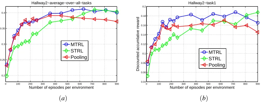
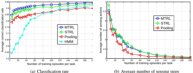
We consider the problem of multi-task reinforcement learning (MTRL) in multiple partially ob-servable stochastic environments. We introduce the regionalized policy representation (RPR) to characterize the agent’s behavior in each environment. The RPR is a parametric model of the con-ditional distribution over current actions given the history of past actions and observations; the agent’s choice of actions is directly based on this conditional distribution, without an interven-ing model to characterize the environment itself. We propose off-policy batch algorithms to learn the parameters of the RPRs, using episodic data collected when following a behavior policy, and show their linkage to policy iteration. We employ the Dirichlet process as a nonparametric prior over the RPRs across multiple environments. The intrinsic clustering property of the Dirichlet process imposes sharing of episodes among similar environments, which effectively reduces the number of episodes required for learning a good policy in each environment, when data sharing is appropriate. The number of distinct RPRs and the associated clusters (the sharing patterns) are automatically discovered by exploiting the episodic data as well as the nonparametric nature of the Dirichlet process. We demonstrate the effectiveness of the proposed RPR as well as the RPR-based MTRL framework on various problems, including grid-world navigation and multi-aspect target classification. The experimental results show that the RPR is a competitive reinforcement learning algorithm in partially observable domains, and the MTRL consistently achieves better performance than single task reinforcement learning.
Keywords: reinforcement learning, partially observable Markov decision processes, multi-task learning, Dirichlet processes, regionalized policy representation
1. Introduction
difficult to meet in practice. In many cases the only knowledge available to the agent are experi-ences, that is, the observations and rewards, resulting from interactions with the environment, and the agent must learn the behavior policy based on such experience. This problem is known as rein-forcement learning (RL) (Sutton and Barto, 1998). Reinrein-forcement learning methods generally fall into two broad categories: model-based and model-free. In model-based methods, one first builds a POMDP model based on experiences and then exploits the existing planning algorithms to find the POMDP policy. In model-free methods, one directly infers the policy based on experiences. The focus of this paper is on the latter, trying to find the policy for a partially observable stochastic environment without the intervening stage of environment-model learning.
In model-based approaches, when the model is updated based on new experiences gathered from the agent-environment interaction, one has to solve a new POMDP planing problem. Solving a POMDP is computationally expensive, which is particularly true when one takes into account the model uncertainty; in the latter case the POMDP state space grows fast, often making it inefficient to find even an approximate solution (Wang et al., 2005). Recent work (Ross et al., 2008) gives a relatively efficient approximate model-based method, but still the computation time grows expo-nentially with the planning horizon. By contrast, model-free methods update the policy directly, without the need to update an intervening POMDP model, thus saving time and eliminating the errors introduced by approximations that may be made when solving the POMDP.
Model-based methods suffer particular computational inefficiency in multi-task reinforcement learning (MTRL), the problem being investigated in this paper, because one has to repeatedly solve multiple POMDPs due to frequent experience-updating arising from the communications among different RL tasks. The work in Wilson et al. (2007) assumes the environment states are perfectly observable, reducing the POMDP in each task to a Markov decision process (MDP); since a MDP is relatively efficient to solve, the computational issue is not serious there. In the present paper, we assume the environment states are partially observable, thus manifesting a POMDP associated with each environment. If model-based methods are pursued, one would have to solve multiple POMDPs for each update of the task clusters, which entails a prohibitive computational burden.
Model-free methods are consequently particularly advantageous for MTRL in partially observ-able domains. The regionalized policy representation (RPR) proposed in this paper, which yields an efficient parametrization for the policy governing the agent’s behavior in each environment, lends itself naturally to a Bayesian formulation and thus furnishes a posterior distribution of the policy. The policy posterior allows the agent to reason and plan under uncertainty about the policy itself. Since the ultimate goal of reinforcement learning is the policy, the policy’s uncertainty is more di-rect and relevant to the learning goal than the POMDP model’s uncertainty as considered in Ross et al. (2008).
environment are scarce (Thrun, 1996). Many problems in practice can be formulated as an MTRL problem, with one example given in Wilson et al. (2007). The application we consider in the exper-iments (see Section 6.2.3) is another example, in which we make the more realistic assumption that the states of the environments are partially observable.
To date there has been much work addressing the problem of inferring the sharing structure between general learning tasks. Most of the work follows a hierarchical Bayesian approach, which assumes that the parameters (models) for each task are sampled from a common prior distribution, such as a Gaussian distribution specified by unknown hyper-parameters (Lawrence and Platt, 2004; Yu et al., 2003). The parameters as well as the hyper-parameters are estimated simultaneously in the learning phase. In Bakker and Heskes (2003) a single Gaussian prior is extended to a Gaussian mixture; each task is given a corresponding Gaussian prior and related tasks are allowed to share a common Gaussian prior. Such a formulation for information sharing is more flexible than a single common prior, but still has limitations: the form of the prior distribution must be specified a priori, and the number of mixture components must also be pre-specified.
In the MTRL framework developed in this paper, we adopt a nonparametric approach by em-ploying the Dirichlet process (DP) (Ferguson, 1973) as our prior, extending the work in Yu et al. (2004) and Xue et al. (2007) to model-free policy learning. The nonparametric DP prior does not assume a specific form, therefore it offers a rich representation that captures complicated sharing patterns among various tasks. A nonparametric prior drawn from the DP is almost surely discrete, and therefore a prior distribution that is drawn from a DP encourages task-dependent parameter clustering. The tasks in the same cluster share information and are learned collectively as a group. The resulting MTRL framework automatically learns the number of clusters, the members in each cluster as well as the associated common policy.
The nonparametric DP prior has been used previously in MTRL (Wilson et al., 2007), where each task is a Markov decision process (MDP) assuming perfect state observability. To the authors’ knowledge, this paper represents the first attempt to apply the DP prior to reinforcement learning in multiple partially observable stochastic environments. Another distinction is that the method here is model-free, with information sharing performed directly at the policy level, without having to learn a POMDP model first; the method in Wilson et al. (2007) is based on using MDP models.
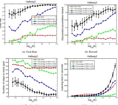
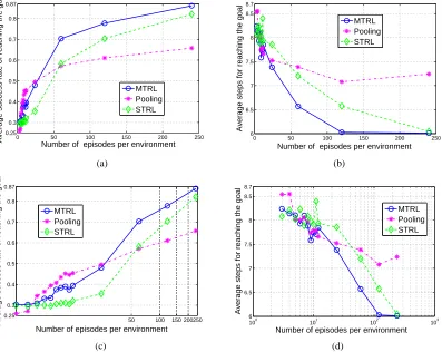
This paper contains several technical contributions. We propose the regionalized policy repre-sentation (RPR) as an efficient parametrization of stochastic policies in the absence of a POMDP model, and develop techniques of learning the RPR parameters based on maximizing the sum of discounted rewards accrued during episodic interactions with the environment. An analysis of the techniques is provided, and relations are established to the expectation-maximization algorithm and the POMDP policy improvement theorem. We formulate the MTRL framework by placing multiple RPRs in a Bayesian setting and employ a draw from the Dirichlet process as their common nonpara-metric prior. The Dirichlet process posterior is derived, based on a nonconventional application of Bayes law. Because the DP posterior involves large mixtures, Gibbs sampling analysis is inefficient. This motivates a hybrid Gibbs-variational algorithm to learn the DP posterior. The proposed tech-niques are evaluated on four problem domains, including the benchmark Hallway2 (Littman et al., 1995), its multi-task variants, and a remote sensing application. The main theoretical results in the paper are summarized in the form of theorems and lemmas, the proofs of which are all given in the Appendix.
2. Partially Observable Markov Decision Processes
The partially observable Markov decision process (POMDP) (Sondik, 1971; Lovejoy, 1991; Kael-bling et al., 1998) is a mathematical model for the optimal control of an agent situated in a partially observable stochastic environment. In a POMDP the state dynamics of the agent are governed by a Markov process, and the state of the process is not completely observable but is inferred from observations; the observations are probabilistically related to the state. Formally, the POMDP can be described as a tuple(
S
,A
,T,O
,Ω,R), whereS
,A
,O
respectively denote a finite set of states, actions, and observations; T are state-transition matrices with Tss′(a)the probability of transiting to state s′ by taking action a in state s; Ωare observation functions with Ωs′o(a) the probability of observing o after performing action a and transiting to state s′; and R is a reward function withR(s,a)the expected immediate reward received by taking action a in state s.
The optimal control of a POMDP is represented by a policy for choosing the best action at any time such that the future expected reward is maximized. Since the state in a POMDP is only partially observable, the action choice is based on the belief state, a sufficient statistic defined as the probability distribution of the state s given the history of actions and observations (Sondik, 1971). It is important to note that computation of the belief state requires knowing the underlying POMDP model.
The belief state constitutes a continuous-state Markov process (Smallwood and Sondik, 1973). Given that at time t the belief state is b and the action a is taken, and the observation received at time t+1 is o, then the belief state at time t+1 is computed by Bayes rule
bao(s′) =∑s∈Sb(s)T a ss′Ωas′o
p(o|b,a) , (1)
where the superscript a and the subscript o are used to indicate the dependence of the new belief state on a and o, and
p(o|b,a) =
∑
s′∈Ss∈∑
Sb(s)Ta
ss′Ωas′o (2)
is the probability of transiting from b to b′when taking action a.
Equations (1) and (2) imply that, for any POMDP, there exists a corresponding Markov deci-sion process (MDP), the state of which coincides with the belief state of the POMDP (hence the term “belief-state MDP”). Although the belief state is continuous, their transition probabilities are discrete : from any given b, one can only make a transition to a finite number of new belief states
{bao: a∈
A
,o∈O
}, assumingA
andO
are discrete sets with finite alphabets. For any action a∈A
, the belief state transition probabilities are given byp(b′|b,a) =
p(o|b,a), if b′=bao
0, otherwise . (3)
The expected reward of the belief-state MDP is given by
R(b,a) =
∑
s∈Sb(s)R(s,a). (4)
In summary, the belief-state MDP is completely defined by the action set
A
, the space of belief stateB
=(
b∈R|S|: b(s)≥0,
∑
s∈S
b(s) =1
)
along with the belief state transition probabilities in (3) and the reward function in (4).
The optimal control of the POMDP can be found by solving the corresponding belief-state MDP. Assume that at any time there are infinite steps remaining for the POMDP (infinite horizon), the future rewards are discounted exponentially with a factor 0<γ<1, and the action is drawn from pΠ(a|b), then the expected reward accumulated over the infinite horizon satisfies the Bellman equation (Bellman, 1957; Smallwood and Sondik, 1973)
VΠ(b) =
∑
a∈A
pΠ(a|b)
"
R(b,a) +γ
∑
o∈Op(o|b,a)VΠ(bao)
#
,
where VΠ(b)is called the value function. Sondik (1978) showed that, for a finite-transient deter-ministic policy,1 there exists a Markov partition
B
=B
1∪B
2∪ · · · satisfying the following two properties :(a) There is a unique optimal action ai associated with subset
B
i, i=1,2,· · ·. This implies thatthe optimal control is represented by a deterministic mapping from the Markov partition to the set of actions.
(b) Each subset maps completely into another (or itself), that is,{bao: b∈
B
i,a=Π(b),o∈O
} ⊆B
j(i may equal j).The Markov partition yields an equivalent representation of the finite-transient deterministic policy. Sondik noted that an arbitrary policyΠis not likely to be finite-transient, and for it one can only construct a partition where one subset maps partially into another (or itself), that is, there exists
b∈
B
iand o∈O
such that boΠ(b)∈/B
j. Nevertheless, the Markov partition provides an approximaterepresentation for non-finite-transient policies and Sondik gave an error bound of the difference between the true value function and approximate value function obtained by the Markov partition. Based on the Markov partition, Sondik also proposed a policy iteration algorithm for POMDPs, which was later improved by Hansen (1997) and the improved algorithm is referred to as finite state controller (the partition is finite).
3. Regionalized Policy Representation
We are interested in model-free policy learning, that is, we assume the model of the POMDP is
unknown and aim to learn the policy directly from the experiences (data) collected from
agent-environment interactions. One may argue that we do in fact learn a model, but our model is directly at the policy level, constituting a probabilistic mapping from the space of action-observation histo-ries to the action space.
Although the optimal control of a POMDP can be obtained via solving the corresponding belief-state MDP, this is not true when we lack an underlying POMDP model. This is because, as indicated above, the observability of the belief-state depends on the availability of the POMDP model. When the model is unknown, one does not have access to the information required to compute the belief state, making the belief state unobservable.
1. LetΠbe a deterministic policy, that is, pΠ(a|b) =
1, if a=Π(b)
0, otherwise . Let S
n
Πbe the set of all possible belief-states
In this paper, we treat the belief-state as a hidden (latent) variable and marginalize it out to yield a stochastic POMDP policy that is purely dependent on the observable history, that is, the sequence of previous actions and observations. The belief-state dynamics, as well as the optimal control in each state, is learned empirically from experiences, instead of being computed from an underlying POMDP model. Although it may be possible to learn the dynamics and control in the continuous space of belief state, the exposition in this paper is restricted to the discrete case, that is, the case for which the continuous belief-state space is quantized into a finite set of disjoint regions. The quantization can be viewed as a stochastic counterpart of the Markov partition (Sondik, 1978), discussed at the end of Section 2. With the quantization, we learn the dynamics of belief regions and the local optimal control in each region, both represented stochastically. The stochasticity manifests the uncertainty arising from the belief quantization (the policy is parameterized in terms of latent belief regions, not the precise belief state). The stochastic policy reduces to a deterministic one when the policy is finitely transient, in which case the quantization becomes a Markov partition. The resulting framework is termed regionalized policy representation to reflect the fact that the policy of action selection is expressed through the dynamics of belief regions as well as the local controls in each region. We also use decision state as a synonym of belief region, in recognition of the fact that each belief region is an elementary unit to encode the decisions of action selection.
3.1 Formal Framework
Definition 1 A regionalized policy representation (RPR) is a tupleh
A
,O
,Z
,W,µ,πi specified as follows. TheA
andO
are respectively a finite set of actions and observations. TheZ
is a finite set of decision states (belief regions). The W are decision-state transition matrices with W(z,a,o′,z′) denoting the probability of transiting from z to z′when taking action a in decision state z results in observing o′. The µ is the initial distribution of decision states with µ(z)denoting the probability of initially being in decision state z. Theπare state-dependent stochastic policies withπ(z,a)denoting the probability of taking action a in decision state z.The stochastic formulation of W andπin Definition 1 is fairly general and subsumes two special cases.
1. If z shrinks down to a single belief-state b, z=b becomes a sufficient statistic of the POMDP
(Smallwood and Sondik, 1973) and there is a unique action associated with it, thusπ(z,a)is deterministic and the local policy can be simplified as a=π(b).
2. If the belief regions form a Markov partition of the belief-state space (Sondik, 1978), that is,
B
=∪z∈ZB
z, then the action choice in each region is constant and one region transitscompletely to another (or itself). In this case, both W andπare deterministic and, moreover, the policy yielded by the RPR (see (8)) is finite transient deterministic. In fact this is the same case as considered in Hansen (1997).
In both of the two special cases, each z has one action choice a=π(z)associated with it, and one can write W(z,a,o′,z′) =W(z,π(z),o′,z′), thus the transition of z is driven solely by o. In general, each z represents multiple individual belief-states, and the belief region transition is driven jointly by a and o. The action-dependency captures the state dynamics of the POMDP, and the observation-dependency reflects the partial observability of the state (perception aliasing).
• The elements of
A
are enumerated asA
={1,2,· · ·,|A
|}, where|A
|denotes the cardinality ofA
. Similarly,O
={1,2,· · ·,|O
|}andZ
={1,2,· · ·,|Z
|}.• A sequence of actions(a0,a1,· · ·,aT)is abbreviated as a0:T, where the subscripts index
dis-crete time steps. Similarly a sequence of observations(o1,o2,· · ·,oT)is abbreviated as o1:T,
and a sequence of decision states(z0,z1,· · ·,zT)is abbreviated as z0:T, etc.
• A history ht is the set of actions executed and observation received up to time step t, that is, ht={a0:t−1,o1:t}.
LetΘ={π,µ,W} denote the parameters of the RPR. Given a history of actions and observa-tions, ht = (a0:t−1,o1:t), collected up to time step t, the RPR yields a joint probability distribution
of z0:t and a0:t
p(a0:t,z0:t|o1:t,Θ) =µ(z0)π(z0,a0) t
∏
τ=1W(zτ−1,aτ−1,oτ,zτ)π(zτ,aτ), (5)
where application of local controlsπ(zt,at) at every time step implies that a0:t are all drawn
ac-cording to the RPR. The decision states z0:t in (5) are hidden variables and we marginalize them to
get
p(a0:t|o1:t,Θ) = |Z|
∑
z0,···,zt=1
"
µ(z0)π(z0,a0) t
∏
τ=1W(zτ−1,aτ−1,oτ,zτ)π(zτ,aτ)
#
. (6)
It follows from (6) that
p(a0:t−1|o1:t,Θ) = |A|
∑
at=1
p(a0:t|o1:t,Θ)
=
|Z|
∑
z0,···,zt−1=1
"
µ(z0)π(z0,a0) t−1
∏
τ=1W(zτ−1,aτ−1,oτ,zτ)π(zτ,aτ)
#
× |A|
∑
at=1
|Z|
∑
zt=1
W(zt−1,at−1,ot,zt)π(zt,at)
| {z }
=1
= p(a0:t−1|o1:t−1,Θ), (7)
which implies that observation ot does not influence the actions before t, in agreement with
expec-tations. From (6) and (7), we can write the history-dependent distribution of action choices
p(aτ|hτ,Θ) = p(aτ|a0:τ−1,o1:τ,Θ) = p(a0:τ|o1:τ,Θ) p(a0:τ−1|o1:τ,Θ)
= p(a0:τ|o1:τ,Θ) p(a0:τ−1|o1:τ−1,Θ)
, (8)
which gives a stochastic RPR policy for choosing the action at, given the historical actions and
ob-servations. The policy is purely history-dependent, with the unobservable belief regions z integrated out.
The history ht forms a Markov process with transitions driven by actions and observations: ht=ht−1∪ {at−1,ot}. Applying this recursively, we get ht=∪tτ=1{aτ−1,oτ}, and therefore
t
∏
τ=0p(aτ|hτ,Θ) =
"
t−2
∏
τ=0p(aτ|hτ,Θ)
#
=
"
t−2
∏
τ=0p(aτ|hτ,Θ)
#
p(at−1:t|ht−1,ot,Θ)
=
"
t−3
∏
τ=0p(aτ|hτ,Θ)
#
p(at−2|ht−2,Θ)p(at−1:t|ht−2,at−2,ot−1,ot,Θ)
=
"
t−3
∏
τ=0p(aτ|hτ,Θ)
#
p(at−2:t|ht−2,ot−1:t,Θ)
.. .
= p(a0:t|h0,o1:t,Θ)
= p(a0:t|o1:t,Θ), (9)
where we have used p(aτ|hτ,oτ+1:t) =p(aτ|hτ) and h0 =null. The rightmost side of (9) is the
observation-conditional probability of joint action-selection at multiple time stepsτ=0,1,· · ·,t.
Equation (9) can be verified directly by multiplying (8) overτ=0,1,· · ·,t
t
∏
τ=0p(aτ|hτ,Θ)
= p(a0|Θ)p(a0:1|o1,Θ) p(a0|Θ)
p(a0:2|o1:2,Θ) p(a0:1|o1,Θ) · · ·
p(a0:t−1|o1:t−1,Θ) p(a0:t−2|o1:t−2,Θ)
p(a0:t|o1:t,Θ) p(a0:t−1|o1:t−1,Θ)
= p(a0:t|o1:t,Θ). (10)
It is of interest to point out the difference between the RPR and previous reinforcement learning algorithms for POMDPs. The reactive policy and history truncation (Jaakkola et al., 1995; Bax-ter and Bartlett, 2001) condition the action only upon the immediate observation or a truncated sequence of observations, without using the full history, and therefore these are clearly different from the RPR. The U-tree (McCallum, 1995) stores historical information along the branches of decision trees, with the branches split to improve the prediction of future return or utility. The draw-back is that the tree may grow intolerably fast with the episode length. The finite policy graphs (Meuleau et al., 1999), finite state controllers (Aberdeen and Baxter, 2002), and utile distinction HMMs (Wierstra and Wiering, 2004) use internal states to memorize the full history, however, their state transitions are driven by observations only. In contrast, the dynamics of decision states in the RPR are driven jointly by actions and observations, the former capturing the dynamics of world-states and the latter reflecting the perceptual aliasing. Moreover, none of the previous algorithms is based on Bayesian learning, and therefore they are intrinsically not amenable to the Dirichlet process framework that is used in the RPR for multi-task examples.
3.2 The Learning Objective
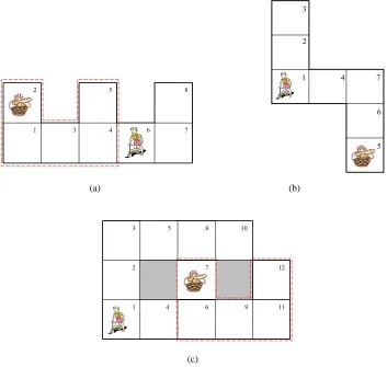
We are interested in empirical learning of the RPR, based on a set of episodes defined as follows.
Definition 2 (Episode) An episode is a sequence of agent-environment interactions terminated in
an absorbing state that transits to itself with zero rewards (Sutton and Barto, 1998). An episode is denoted by(ak
0rk0ok1a1krk1· · ·okTka
k Tkr
k
Tk), where the subscripts are discrete times, k indexes the episodes,
Definition 3 (Sub-episode) A sub-episode is an episode truncated at a particular time step and
retaining the immediate reward only at the time step where truncation occurs. The t-th sub-episode of episode(ak
0r0kok1a1krk1· · ·okTka
k Tkr
k
Tk) is defined as(a
k
0ok1ak1· · ·otkatkrtk), which yields a total of Tk+1 sub-episodes for this episode.
The learning objective is to maximize the optimality criterion given in Definition 4. Theorem 5 introduced below establishes the limit of the criterion when the number of episodes approaches infinity.
Definition 4 (The RPR Optimality Criterion) Let
D
(K)={(ak0rk0ok1a1krk1· · ·okTka
k Tkr
k Tk)}
K
k=1 be a set of episodes obtained by an agent interacting with the environment by following policyΠto select actions, whereΠis an arbitrary stochastic policy with action-selecting distributions pΠ(at|ht)>0,
∀action at,∀history ht. The RPR optimality criterion is defined as
b
V(
D
(K);Θ)de f=. 1 KK
∑
k=1 Tk
∑
t=0
γtrk t
∏t
τ=0pΠ(akτ|hkτ) t
∏
τ=0p(ak
τ|hkτ,Θ), (11)
where hkt =ak0o1kak1· · ·okt is the history of actions and observations up to time t in the k-th episode,
0<γ<1 is the discount, andΘdenotes the parameters of the RPR.
Theorem 5 LetVb(
D
(K);Θ)be as defined in Definition 4, then limK→∞Vb(D
(K);Θ)is the expected sum of discounted rewards within the environment under test by following the RPR policy parame-terized byΘ, over an infinite horizon.Theorem 5 shows that the optimality criterion given in Definition 4 is the expected sum of discounted rewards in the limit, when the number of episodes approaches infinity. Throughout the paper, we call limK→∞Vb(
D
(K);Θ)the value function andVb(D
(K);Θ)the empirical value function.TheΘmaximizing the (empirical) value function is the best RPR policy (given the episodes). It is assumed in Theorem 5 that the behavior policy Πused to collect the episodic data is an arbitrary policy that assigns nonzero probability to any action given any history, that is,Πis required to be a soft policy (Sutton and Barto, 1998). This premise assures a complete exploration of the actions that might lead to large immediate rewards given any history, that is, the actions that might be selected by the optimal policy.
4. Single-Task Reinforcement Learning (STRL) with RPR
We develop techniques to maximize the empirical value function in (11) and theΘresulting from value maximization is called a Maximum-Value (MV) estimate (related to maximum likelihood). An MV estimate of the RPR is preferred when the number of episodes is large, in which case the empirical value function approaches the true value function and the estimate is expected to approach the optimal (assuming the algorithm is not trapped in a local minima). The episodes
D
(K)are assumed to have been collected in a single partially observable stochastic environment, which may correspond to a single physical environment or a pool of multiple identical/similar physical environments. As a result, the techniques developed in this section are for single-task reinforcement learning (STRL).
b
V(
D
(K);Θ) = 1 KK
∑
k=1 Tk
∑
t=0
˜rtk
|Z|
∑
zk
0,···,zkt=1
p(ak0:t,zk0:t|ok1:t,Θ), (12)
where
˜rtk= γ trk
t
∏t
τ=0pΠ(akτ|hkτ)
is the discounted immediate rewardγtrtkweighted by the inverse probability that the behavior policy
Π has generated rtk. The weighting is a result from importance sampling (Robert and Casella, 1999), and reflects the fact that rtkis obtained by followingΠbut the Monte Carlo integral (i.e., the empirical value function) is with respect to the RPR policyΘ. For simplicity, ˜rtk is also referred to as discounted immediate reward or simply reward throughout the paper.
We assume rt ≥0 (and henceert ≥0), which can always be achieved by adding a constant to rt;
this results in a constant added to the value function (the value function of a POMDP is linear in immediate reward) and does not influence the policy.
Theorem 6 (Maximum Value Estimation) Let
qtk(zk0:t|Θ(n)) = ˜r k t
b
V(
D
(K);Θ(n))p(ak
0:t,zk0:t|o1:tk ,Θ(n)), (13) for zk
t =1,2,· · ·,|
Z
|, t=1,2,· · ·,Tk, and k=1,2,· · ·,K. LetΘ(n+1)=arg max b Θ∈F
1
K K
∑
k=1 Tk
∑
t=0 |Z|
∑
zk
0,···,zkt=1
qkt(zk0:t|Θ(n))ln˜r
k
tp(ak0:t,zk0:t|ok1:t,Θb) qtk(zk0:t|Θ(n))
, (14)
where
F
=(
Θ= (µ,π,W):
|Z|
∑
j=1
b
µ(j) =1,
|A|
∑
a=1
b
π(i,a) =1,
|Z|
∑
j=1
b
W(i,a,o,j) =1,
i=1,2,· · ·,|
Z
|,a=1,2,· · ·,|A
|,o=1,2,· · ·,|O
|)
is the set of feasible parameters for the RPR in question. Let{Θ(0)Θ(1)· · ·Θ(n)· · · }be a sequence
yielded by iteratively applying (13) and (14), starting fromΘ(0). Then
lim
n→∞Vb(
D
(K);Θ(n))
exists and the limit is a maxima ofVb(
D
(K);Θ).To gain a better understanding of Theorem 6, we rewrite (13) to get
qkt(zk0:t|Θ) = σ k t(Θ)
b
V(
D
(K);Θ)p(zk
where p(zk
0:t|ak0:t,ok1:t,Θ)is an standard posterior distribution of the latent decision states given the
Θupdated in the most recent iteration (the superscript(n)indicating the iteration number has been dropped for simplicity), and
σk t(Θ)
De f.
= ˜rtkp(ak0:t|ok1:t,Θ) (16)
is called the re-computed reward at time step t in the k-th episode. The re-computed reward rep-resents the discounted immediate reward ˜rtk weighted by the probability that the action sequence
yielding this reward is generated by the RPR policy parameterized byΘ, thereforeσkt(Θ)is a func-tion of Θ. The re-computed reward reflects the update of the RPR policy which, if allowed to re-interact with the environment, is expected to accrue larger rewards than in the previous iteration. Recall that the algorithm does not assume real re-interactions with the environment so the episodes themselves cannot update. However, by recomputing the rewards as in (16), the agent is allowed to generate an internal set of episodes in which the immediate rewards are modified. The internal episodes represent the new episodes that would be collected if the agent followed the updated RPR to really re-interact with the environment. In this sense, the reward re-computation can be thought of as virtual re-interactions with the environment.
By (15), qkt(zk
0:t)is a weighted version of the standard posterior of zk0:t, with the weight given by
the reward recomputed by the RPR in the previous iteration. The normalization constantVb(
D
(K);Θ), which is also the empirical value function in (11), can be expressed as the recomputed rewards av-eraged over all episodes at all time steps,b
V(
D
(K);Θ) = 1 KK
∑
k=1 Tk
∑
t=0
σk
t(Θ), (17)
which ensures
1
K K
∑
k=1 Tk
∑
t=0 |Z|
∑
zk
0,···,zkt=1
qkt(zk0:t|Θ) =1.
The maximum value (MV) algorithm based on alternately applying (13) and (14) in Theorem 6 bears strong resemblance to the expectation-maximization (EM) algorithms (Dempster et al., 1977) widely used in statistics, with (13) and (14) respectively corresponding to the E-step and M-step in EM. However, the goal in standard EM algorithms is to maximize a likelihood function, while the goal of the MV algorithm is to maximize an empirical value function. This causes significant differ-ences between the MV and the EM. It is helpful to compare the MV algorithm in Theorem 6 to the EM algorithm for maximum likelihood (ML) estimation in hidden Markov models (Rabiner, 1989), since both deal with sequences or episodes. The sequences in an HMM are treated as uniformly important, therefore parameter updating is based solely on the frequency of occurrences of latent states. Here the episodes are not equally important because they have different rewards associated with them, which determine their importance relative to each other. As seen in (15), the posterior of zk0:t is weighted by the recomputed rewardσkt, which means that the contribution of episode k (at time t) to the update ofΘis not solely based on the frequency of occurrences of zk0:t but also based on the associatedσk
t. Thus the new parametersΘb will be adjusted in such a way that the episodes
The objective function being maximized in (14) enjoys some interesting properties due to the fact that qkt(zk
0:t)is a weighted posterior of zk0:t. These properties not only establish a more formal
connection between the MV algorithm here and the traditional ML algorithm based on EM, they also shed light on the close relations between Theorem 6 and the policy improvement theorem of POMDP (Blackwell, 1965). To show these properties, we rewrite the objective function in (14) (with the subscript(n)dropped for simplicity) as
LB(Θb|Θ)De f=. 1 K
K
∑
k=1 Tk
∑
t=0 |Z|
∑
zk0,···,zkt=1
qkt(zk 0:t|Θ)ln
˜rtkp(ak
0:t,zk0:t|ok1:t,Θb) qkt(zk0:t|Θ)
= 1
K K
∑
k=1 Tk
∑
t=0
σk t(Θ)
b
V(
D
(K);Θ)|Z|
∑
zk
0,···,zkt=1
p(zk
0:t|ak0:t,ok1:t,Θ)ln
˜rtkp(ak
0:t,zk0:t|ok1:t,Θb)
σk t(Θ)
b
V(D(K);Θ)p(z
k
0:t|ak0:t,ok1:t,Θ)
, (18)
where the second equation is obtained by substituting (15) into the left side of it. Since
1 K∑
K k=1∑
Tk
t=0
σk t(Θ)
b
V(D(K);Θ)=1 and∑
|Z|
zk0,···,zkt=1p(z
k
0:t|ak0:t,ok1:t,Θ) =1, one can apply Jensen’s inequality twice to the rightmost side of (18) to obtain two inequalities
LB(Θb|Θ) ≤ 1 K
K
∑
k=1 Tk
∑
t=0
σk t(Θ)
b
V(
D
(K);Θ)ln˜rtkp(ak
0:t|ok1:t,Θb)
σk t(Θ)
b
V(D(K);Θ)
De f.
= ϒ(Θb|Θ)
≤ ln " 1 K K
∑
k=1 Tk
∑
t=0
˜rtkp(ak
0:t|ok1:t,Θb)
#
= lnVb(
D
(K);Θb), (19)where the first inequality is with respect to p(zk
0:t|ak0:t,ok1:t,Θ) while the second inequality is with
respect to n σkt(Θ)
b
V(D(K);Θ): t=1,· · ·,Tk,k=1,· · ·,K o
. Each inequality yields a lower bound to the
logarithmic empirical value function lnVb(
D
(K);Θb). It is not difficult to verify from (18) and (19) that both of the two lower bounds are tight (the respective equality can be reached), that is,LB(Θ|Θ) =lnVb(
D
(K);Θ) =ϒ(Θ|Θ). (20)The equations in (20) along with the inequalities in (19) show that any Θb satisfying LB(Θ|Θ)<
LB(Θb|Θ) orϒ(Θ|Θ)<ϒ(Θb|Θ)also satisfiesVb(
D
(K);Θ)<Vb(D
(K);Θb). Thus one can choose tomaximize either of the two lower bounds, LB(Θb|Θ)orϒ(Θb|Θ), when trying to improve the empir-ical value ofΘb over that ofΘ. In either case, the maximization is with respect toΘb.
The two alternatives, though both yielding an improved RPR, are quite different in the manner the improvement is achieved. Suppose one has obtainedΘ(n)by applying (13) and (14) for n itera-tions, and is seekingΘ(n+1)satisfyingVb(
D
(K);Θ(n))<Vb(D
(K);Θ(n+1)). Maximization of the first lower bound givesΘ(n+1)=arg maxΘb∈FLB(Θb|Θ(n)), which has an analytic solution that will begiven in Section 4.2. Maximization of the second lower bound yields
Θ(n+1)=arg max b Θ∈F
ϒ(Θb|Θ(n)). (21)
The definition ofϒin (19) is substituted into (21) to yield
Θ(n+1) = arg max b Θ∈F
1
K K
∑
k=1 Tk
∑
t=0
σk t(Θ(n))
b
V(
D
(K);Θ(n))ln˜rtkp(ak
0:t|ok1:t,Θb)
σk t(Θ(n))
b
= arg max
b Θ∈F
K
∑
k=1 Tk
∑
t=0
σk
t(Θ(n))ln p(a0:tk |ok1:t,Θb), (22)
which shows that maximization of the second lower bound is equivalent to maximizing a weighted sum of the log-likelihoods of {ak0:t}, with the weights being the rewards recomputed by Θ(n). Through (22), the connection between the maximum value algorithm in Theorem 6 and the tra-ditional ML algorithm is made more formal and clearer: with the recomputed rewards given and fixed, the MV algorithm is a weighted version of the ML algorithm, with ϒ(Θb|Θ(n)) a weighted
log-likelihood function ofΘb.
The above analysis also sheds light on the relations between Theorem 6 and the policy improve-ment theorem in POMDP (Blackwell, 1965). By (19), (20), and (22), we have
lnV(
D
(K);Θ(n)) =ϒ(Θ(n)|Θ(n)) ≤ ϒ(Θ(n+1)|Θ(n)) ≤ lnV(D
(K);Θ(n+1)).The first inequality, achieved by the weighted likelihood maximization in (22), represents the policy improvement on the old episodes collected by following the previous policy. The second inequality ensures that, if the improved policy is followed to collect new episodes in the environment, the expected sum of newly accrued rewards is no less than that obtained by following the previous policy. This is similar to policy evaluation. Note that the update of episodes is simulated by reward computation. The actual episodes are collected by a fixed behavior policyΠand do not change.
The maximization in (22) can be performed using any optimization techniques. As long as the maximization is achieved, the policy is improved as guaranteed by Theorem 6. Since the latent z variables are involved, it is natural to employ EM to solve the maximization. The EM solution to (22) is obtained by solving a sequence of maximization problems: starting fromΘ(n)(0)=Θ(n), one
successively solves
Θ(n)(j)=arg max b Θ∈F
LB(Θb|Θ(n)(j−1)) subject toσkt(Θ(n)(j−1)) =σkt(Θ(n)),∀t,k, (23)
j=1,2,· · ·,
where in each problem one maximizes the first lower bound with an updated posterior of {ztk}
but with the recomputed rewards fixed at {σk
t(Θ(n))}; upon convergence, the solution of (23) is
the solution to (22). The EM solution here is almost the same as the likelihood maximization of sequences for hidden Markov models (Rabiner, 1989). The only difference is that here we have a weighted log-likelihood function, but with the weights given and fixed. The posterior of{zkt}can be updated by employing the dynamical programming techniques similar to those used in HMM, as we discuss below.
It is interesting to note that, with standard EM employed to solve (22), the overall maximum value algorithm is a “double-EM” algorithm, since reward computation constitutes an outer EM-like loop.
4.1 Calculating the Posterior of Latent Belief Regions
To allocate the weights or recomputed rewards and update the RPR as in (14), we do not need to know the full distribution of zk0:t. Instead, a small set of marginals of p(zk
for the purpose, in particular,
ξk
t,τ(i,j) = p(zkτ=i,zkτ+1= j|ak0:t,ok1:t,Θ), (24)
φk
t,τ(i) = p(zkτ=i|ak0:t,ok1:t,Θ). (25)
Lemma 7 (Factorization of theξandφVariables) Let
αk
τ(i) = p(zkτ=i|a0:kτ,ok1:τ,Θ)
= p(z
k
τ=i,ak0:τ|ok1:τ,Θ)
∏ττ′=0p(akτ′|hkτ′,Θ)
, (26)
βk
t,τ(i) =
p(ak
τ+1:t|zkτ=i,akτ,okτ+1:t,Θ)
∏t
τ′=τp(akτ′|hkτ′,Θ)
. (27)
Then
ξk
t,τ(i,j) = αkτ(i)W(zkτ=i,akτ,okτ+1,zkτ+1= j)π(zkτ+1= j,aτk+1)βkt,τ+1(j), (28)
φk
t,τ(i) = αkτ(i)βkt,τ(i)p(akτ|hkτ). (29)
The α and βvariables in the Lemma 7 are similar to the scaled forward variables and back-ward variables in hidden Markov models (HMM) (Rabiner, 1989). The scaling factors here are
∏ττ′=0p(akτ′|hkτ′,Θ), which is equal to p(ak0:τ|ok1:τ,Θ)as shown in (9) and (10). Recall from Defini-tion 3 that one episode of length T has T+1 sub-episodes with each having a different ending time step. For this reason, one must compute theβvariables for each sub-episode separately, since the
βvariables depend on the ending time step. Forαvariables, one needs to compute them once per episode, since it does not involve the ending time step.
Similar to the forward variables and backward variables in HMM models, theαandβvariables can be computed recursively, via dynamical programming,
αk
τ(i) =
µ(zk
0=i)π(zk0=i,ak0) p(ak
0|hk0,Θ)
, τ=0
∑|Z|
j=1αkτ−1(j)W(zkτ−1= j,akτ−1,okτ,zkτ=i)π(zkτ=i,akτ) p(ak
τ|hkτ,Θ) , τ>0
, (30)
βk t,τ(i) =
1
p(ak t|hkt,Θ)
, τ=t
∑|Z|
j=1W(zkτ=i,aτk,okτ+1,zkτ+1=j)π(zkτ+1= j,aτk+1)βkt,τ+1(j) p(ak
τ|hkτ,Θ) , τ<t
, (31)
for t=0,· · ·,Tkand k=1,· · ·,K. Since∑|iZ=|1αkτ(i) =1, it follows from (30) that
p(akτ|hkτ,Θ) =
|Z|
∑
i=1
µ(zk0=i)π(zk0=i,ak0), τ=0
|Z|
∑
i=1 |Z|
∑
j=1
αk
τ−1(j)W(zkτ−1= j,akτ−1,okτ,zkτ=i)π(zkτ=i,akτ), τ>0
4.2 Updating the Parameters
We rewrite the lower bound in (18),
LB(Θb|Θ) = 1 K
K
∑
k=1 Tk
∑
t=0 |Z|
∑
zk
0,···,zkt=1
qkt(zk0:t|Θ(n))ln˜r
k
tp(ak0:t,zk0:t|ok1:t,Θb) qk
t(zk0:t|Θ(n))
= 1
K K
∑
k=1 Tk
∑
t=0 |Z|
∑
zk
0,···,zkt=1
qkt(zk0:t|Θ(n))ln p(a0:tk ,zk0:t|ok1:t,Θb) +constant,
where the “constant” collects all the terms irrelevant toΘb. Substituting (5) and (15) gives
LB(Θb|Θ) = 1 K
K
∑
k=1 Tk
∑
t=0
σk t
b
V(
D
(K);Θ) (|Z|∑
i=1
φk
t,0(i)lnbµ(i) + t
∑
τ=0|Z|
∑
i=1
φk
t,τ(i)lnbπ(i,akτ)
+ t
∑
τ=1|Z|
∑
i,j=1
ξk
t,τ(i,j)lnWb(i,akτ−1,okτ,j)
)
+constant.
It is not difficult to show thatΘb=arg maxΘb∈FLB(Θb|Θ)is given by
bµ(i) = ∑
K k=1∑
Tk
t=0σktφtk,0(i)
∑|Z|
i=1∑Kk=1∑ Tk
t=0σktφkt,0(i)
, (33)
b
π(i,a) = ∑
K k=1∑
Tk
t=0σkt∑tτ=0φtk,τ(i)δ(akτ,a) ∑|A|
a=1∑Kk=1∑ Tk
t=0σkt∑tτ=0φkt,τ(i)δ(akτ,a)
, (34)
b
W(i,a,o,j) = ∑ K k=1∑
Tk
t=0σkt∑tτ−1=1ξkt,τ(i,j)δ(akτ,a)δ(okτ+1,o)
∑|Z|
j=1∑Kk=1∑ Tk
t=0σkt ∑t−1τ=1ξkt,τ(i,j)δ(akτ,a)δ(okτ+1,o)
, (35)
for i,j=1,2,· · ·,|
Z
|, a=1,· · ·,|A
|, and o=1,· · ·,|O
|, whereδ(a,b) =
1, a=b
0, a6=b , andσ k t is
the recomputed reward as defined in (16). In computingσkt one employs the equation p(ak
0:t|ok1:t,Θ) =
∏t
τ=0p(akτ|hkτ,Θ)established in (9) and (10), to get
σk t(Θ)
De f.
= ˜rtk
t
∏
τ=0p(akτ|hkτ,Θ), (36)
with p(ak
τ|hkτ,Θ)computed from theαvariables by using (32). Note that the normalization constant, which is equal to the empirical valueVb(
D
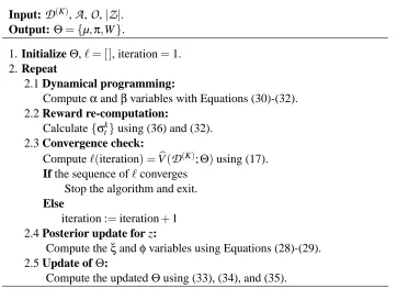
(K);Θ), is now canceled in the update formulae ofΘb.4.3 The Complete Value Maximization Algorithm for Single-Task RPR Learning
The complete value maximization algorithm for single-task RPR learning is summarized in Table 1. In earlier discussions regarding the relations of the algorithm to EM, we have mentioned that reward computation constitutes an outer EM-like loop; the standard EM employed to solve (22) is embedded in the outer loop and constitutes an inner EM loop. The double EM loops are not explicitly shown in Table 1. However, one may separate these two loops by keeping{σk
Input:
D
(K),A
,O
,|Z
|. Output:Θ={µ,π,W}.1. InitializeΘ,ℓ= [ ], iteration=1. 2. Repeat
2.1 Dynamical programming:
Computeαandβvariables with Equations (30)-(32). 2.2 Reward re-computation:
Calculate{σk
t}using (36) and (32).
2.3 Convergence check:
Computeℓ(iteration) =Vb(
D
(K);Θ)using (17). If the sequence ofℓconvergesStop the algorithm and exit. Else
iteration :=iteration+1 2.4 Posterior update for z:
Compute theξandφvariables using Equations (28)-(29). 2.5 Update ofΘ:
Compute the updatedΘusing (33), (34), and (35).
Table 1: The value maximization algorithm for single-task RPR learning
when updatingΘand the posterior of z’s, until the empirical value converges; see (23) for details. Once {σk
t} are updated, the empirical value will further increase by continuing updating Θ and
the posterior of z’s. Note that the{σk
t}used in the convergence check are always updated at each
iteration, even though the new{σk
t}may not be used for updatingΘand the posterior of z’s.
Given a history of actions and observations(a0:t−1,o1:t)collected up to time step t, the single
RPR yields a distribution of at as given by (8). The optimal choice for at can be obtained by either
sampling from this distribution or taking the action that maximizes the probability.
4.3.1 TIMECOMPLEXITYANALYSIS
We quantify the time complexity by the number of real number multiplications performed per it-eration and present it in the Big-O notation. Since there is no compelling reason for the number of iterations to depend on the size of the input,2 the complexity per iteration also represents the complexity of the complete algorithm. A stepwise analysis of the time complexity of the value maximization algorithm in Table 1 is given as follows.
• Computation of theαvariables with (30) and (32) runs in time O(|
Z
|2∑K k=1Tk). • Computation ofβ’s with (31) and (32) runs in time O(|Z
|2∑Kk=1∑ Tk
t=0,rk
t6=0(t+1)), which de-pends on the degree of sparsity of the immediate rewards{rk0rk2· · ·rkTk}K
k=1. In the worst case 2. The number of iterations usually depends on such factors as initialization of the algorithm and the required accuracy,
the time is O(|
Z
|2∑K k=1∑Tk
t=0(t+1)) =O(|
Z
|2∑Kk=1Tk2), which occurs when the immediatere-ward in each episode is nonzero at every time step. In the best case the time is O(|
Z
|2∑K k=1Tk),which occurs when the immediate reward in each episode is nonzero only at a fixed number of time steps (only at the last time step, for example, as is the case of the benchmark problems presented in Section 6).
• The reward re-computation using (36) and (32) requires time O(∑K
k=1Tk) in the worst case
and O(K)in the best case, where the worse/best cases are as defined above.
• Update ofΘusing (33), (34), and (35), as well as computation of theξandφvariables using (28) and (29), runs in time O(|
Z
|2∑Kk=1Tk2)in the worst case and O(|
Z
|2∑Kk=1Tk)in the bestcase, where the worse/best cases are defined above.
Since∑Kk=1Tk≫ |
A
||O
|in general, the overall complexity of the value maximization algorithm isO(|
Z
|2∑Kk=1Tk2) in the worst case and O(|
Z
|2∑ Kk=1Tk) in the best case, depending on the degree
of sparsity of the immediate rewards. Therefore the algorithm scales linearly with the number of episodes and to the square of the number of belief regions. The time dependency on the lengths of episodes is between linear and square. The sparser the immediate rewards are, the more the time is towards being linear in the lengths of episodes.
Note that in many reinforcement problems, the agent does not receive immediate rewards at ev-ery time step. For the benchmark problems and maze navigation problems considered in Section 6, the agent receives rewards only when the goal state is reached, which makes the value maximization algorithm scale linearly with the lengths of episodes.
5. Multi-Task Reinforcement Learning (MTRL) with RPR
We formulate our MTRL framework by placing multiple RPRs in a Bayesian setting and develop techniques to learn the posterior of each RPR within the context of all other RPRs.
Several notational conventions are observed in this section. The posterior ofΘis expressed in terms of probability density functions. The notation G0(Θ)is reserved to denote the density function of a parametric prior distribution, with the associated probability measure denoted by G0without a
parenthesizedΘbeside it. For the Dirichlet process (which is a nonparametric prior), G0 denotes
the base measure and G0(Θ) denotes the corresponding density function. The twofold use of G0
is for notational simplicity; the difference can be easily discerned by the presence or absence of a parenthesizedΘ. Theδis a Dirac delta for continuous arguments and a Kronecker delta for discrete
arguments. The notationδΘj is the Dirac measure satisfyingδΘj(dΘm) =
1, Θj∈dΘm
0, otherwise .
5.1 Basic Bayesian Formulation of RPR
Consider M partially observable and stochastic environments indexed by m=1,2· · ·,M, each of
which is apparently different from the others but may actually share fundamental common char-acteristics with some other environments. Assume we have a set of episodes collected from each
environment,
D
(Km)m =
n
(am0,kr0m,kom1,kam1,krm1,k· · ·omT,k
m,ka
m,k Tm,kr
m,k Tm,k)
oKm
k=1, for m=1,2,· · ·,M, where Tm,k
write the empirical value function of the m-th environment as
b
V(
D
(Km)m ;Θm) =
1
Km Km
∑
k=1 Tm,k
∑
t=0
˜rmt ,kp(am0:t,k|o m,k
1:t ,Θm), (37)
for m=1,2,· · ·,M, where Θm ={πm,µm,Wm} are the RPR parameters for the m-th individual
environment.
Let G0(Θm)represent the prior ofΘm, where G0(Θ)is assumed to be the density function of a
probability distribution. We define the posterior ofΘmas
p(Θm|
D
m(Km),G0) De f.= Vb(
D
(Km)
m ;Θm)G0(Θm)
b
VG0(
D
(Km)
m )
, (38)
where the inclusion of G0in the left hand side is to explicitly indicate that the prior being used is G0, andVbG0(
D
(Km)
m )is a normalization constant
b
VG0(
D
(Km)
m ) De f.
=
Z
b
V(
D
(Km)m ;Θm)G0(Θm)dΘm, (39)
which is also referred to as the marginal empirical value,3since the parametersΘmare integrated out
(marginalized). The marginal empirical valueVGb 0(
D
(Km)
m ) represents the accumulated discounted
reward in the episodes, averaged over infinite RPR policies independently drawn from G0.
Equation (38) is literally a normalized product of the empirical value function and a prior
G0(Θm). Since
R
p(Θm|
D
( Km)m ,G0)dΘm=1, (38) yields a valid probability density, which we call
the posterior of Θm given the episodes
D
m(Km). It is noted that (38) would be the Bayes rule ifb
V(
D
(Km)m ;Θm)were a likelihood function. SinceVb(
D
( Km)m ;Θm)is a value function in our case, (38)
is a somewhat non-standard use of Bayes rule. However, like the classic Bayes rule, (38) indeed gives a posterior whose shape incorporates both the prior information aboutΘmand the empirical
information from the episodes.
Equation (38) has another interpretation that may be more meaningful from the perspective of standard probability theory. To see this we substitute (37) into (38) to obtain
p(Θm|
D
m(Km),G0) = 1 Km∑Km
k=1∑ Tm,k
t=0˜r m,k
t p(am0:t,k|o m,k
1:t ,Θm)G0(Θm)
b
VG0(
D
(Km)
m )
(40)
= 1 Km∑
Km
k=1∑ Tm,k
t=0ζ m,k
t p(Θm|am0:t,k,o m,k 1:t ,G0)
b
VG0(
D
(Km)
m )
, (41)
where
ζm,k
t = ˜r m,k t p(a
m,k 0:t |o
m,k 1:t ,G0) = ˜rtm,k
Z
p(am0:t,k|om1:t,k,Θm)G0(Θm)dΘm =
Z
σm,k
t (Θm)G0(Θm)dΘm, (42) 3. The term “marginal” is borrowed from the probability theory. Here we use it to indicate that the dependence of the
withσmt ,kthe re-computed reward as defined in (16) and thereforeζtm,kis the averaged re-computed
reward, obtained by taking the expectation ofσmt ,k(Θm)with respect to G0(Θm).
In arriving (41), we have used the fact the RPR parameters are independent of the observations, which is true due to the following reasons: RPR is a policy concerning generation of the actions, employing as input the observations (which themselves are generated by the unknown environment); therefore, observations carry no information about the RPR parameters, that is, p(Θ|observations) = p(Θ)≡G0(Θ).
It is noted that p(Θm|am0:t,k,o m,k
1:t ,G0) in (41) is the standard posterior of Θm given the action
sequence am0:t,k, and p(Θm|
D
m(Km),G0) is a mixture of these posteriors with the mixing proportiongiven byζmt ,k. The meaning of (40) is fairly intuitive: each action sequence affects the posterior of
Θmin proportion to its re-evaluated reward. This is distinct from the posterior in the classic hidden
Markov model (Rabiner, 1989) where sequences are treated as equally important. Since p(Θm|
D
(Km)
m ,G0)integrates to one, the normalization constantVbG0(
D
(Km)
m )is
b
VG0(
D
(Km)
m ) =
1
Km Km
∑
k=1 Tm,k
∑
t=0
ζm,k
t . (43)
We obtain a more convenient form of the posterior by substituting (6) into (41) to expand the summation over the latent z variables, yielding
p(Θm|
D
m(Km),G0) = 1 Km∑Km
k=1∑ Tm,k
t=0˜r m,k t ∑
|Z|
zm0,k,···,zmt,k=1
p(am0:t,k,zm0:t,k|om1:t,k,Θm)G0(Θm)
b
VG0(
D
(Km)
m )
. (44)
To obtain an analytic posterior, we let the prior be conjugate to p(am0:t,k,z0:tm,k|om1:t,k,Θm). As shown
by (5), p(am0:t,k,z0:tm,k|om1:t,k,Θm) is a product of multinomial distributions, and hence we choose the prior as a product of Dirichlet distributions, with each Dirichlet representing an independent prior for a subset of parameters inΘ. The density function of such a prior is given by
G0(Θm) = p(µm|υ)p(πm|ρ)p(Wm|ω), (45)
p(µm|υ) = Dir
µm(1),· · ·,µm(|
Z
|)υ
, (46)
p(πm|ρ) = |Z|
∏
i=1
Dir
πm(i,1),· · ·,πm(i,|
A
|)ρi
, (47)
p(Wm|ω) = |A|
∏
a=1 |O|
∏
o=1 |Z|
∏
i=1
Dir
Wm(i,a,o,1),· · ·,Wm(i,a,o,|
Z
|)ωi,a,o
, (48)
whereυ={υ1, . . . ,υ|Z|},ρ={ρ1, . . . ,ρ|Z|}withρi={ρi,1, . . . ,ρi,|A|}, andω={ωi,a,o: i=1. . .|
Z
|, a=1. . .|A
|,o=1. . .|O
|}withωi,a,o={ωi,a,o,1, . . . ,ωi,a,o,|Z|}. Substituting the expression of G0into (44), one gets
p(Θm|
D
m(Km),G0)= 1 Km∑
Km
k=1∑ Tm,k
t=0∑ |Z|
zm0,k,···,zmt,k=1
ζm,k
t (zm0:t,k)p(Θm|a m,k 0:t ,o
m,k 1:t ,z
m,k 0:t ,G0)
b
VG0(
D
(Km)
m )