Survey of Money- Output Causality: Case Study of Iran,
Based on Vector Error Correction Model (VECM)
Monireh Motamedi Ghazaleh Mohammadian Received: 2014/10/05 Accepted: 2014/12/19
Abstract
his study investigated the dynamic relationship between money, prices and output in a multivariate structure of casualty analysis in Iran for the two period of 1969 to 2012 (entire period) and 1989 to 2012 (sub-period). This statistical framework has been projected for situations where causal links may have changed over the sample period. Results of a three-variable Vector Error Correction Model (VECM) analysis were indicative for existence of one co-integrated relationship between money supply, price and real output at both periods. Although there was a long run relationship between money, output and prices for both periods, direction of casualty has changed for sub-period. Also error correction terms showed that short run adjustment toward long run equilibrium was faster and stranger at sub-period, when Central Bank of Iran (CBI) adopted expansionary monetary policy and consequently rapid increase in liquidity. Finally money- output causality was not confirmed in this method and presence of correlation (not causality) between variables may just resulted from some other variables in economy as source of changes.
Keywords: Monetary Policy, Error Correction Model, Granger Causality, Variance Decomposition, Money-Output Relationship
1-
Introduction
Causality between money and output is one of the most important issues in macroeconomic policy and large literature has examined the relationships between monetary variables and output. Various economic assumptions about money –output relationship, essentially lead to different
Ph.D. in Economics, Monetary and Banking Research Institute (MBRI), Tehran, Iran (Corresponding Author).
Ph.D. Candidate, School of Computer Science, Engineering and Mathematics, Flinders University, Australia.
macroeconomic paradigms. This relationship are historically associated with the quantity theory of money and according to the classical doctrine. They believe that an increase in money supply result only in a relative increase in price in the long-run, on the other hand money is neutral to output. The Keynesians believed that a positive monetary shock would increase both economic activity and price level through the interest rate and investment variables. The Monetarists argue that the Keynesian transmission channel is valid only in the short run, but in the long run classical opinion is valid. The new classical argue that only unanticipated monetary expansion would result in an increase in output. According to the new Keynesians, money is non-neutral at least in the short run, because of rigidities in prices and wages, and market failures and imperfections. The theory of Real Business Cycle (RBC) presume that the money supply is determined endogenously by the circumstances of the economy, not by the central bank and also output is determined exogenously by technology. They argue that money supply endogenously responding to an increase in output, thus monetary expansion will have no positive effect on output and will only raise interest rates and the price level [1]. It is important to mention that, if there is a positive correlation exists between nominal money and real output but as a general rule, correlation is frequently taken to imply causality [2].Then issue implied above by the existing macroeconomic paradigms is still an empirical one.
This paper contributes to the literature based on previous applied studies such Fahlino [3].Our study has been fallowed in a multivariate framework and within the environment of vector error-correction model (VECM).This method was employed to determine the Granger causality among variables to indicate the direction of causality. Since the result of causality tests seem to be sensitive with respect to the sample period, we intend to apply a method of analyzing these causal relatives for Iranian economy in two periods. This viewpoint is considered for the first time between money-output Causality. For this purpose we introduce two different sample, the entire period of 1969-2012 and sub-period or after war period of 1989- 2012, at which central bank`s monetary policy has changed. In this new viewpoint by applying data from central bank of Iran for two period, sensitivity of results with respect to change in sample period is examined.
discusses the empirical-based studies available on the relationship between these variables. Section 3 provides a brief history of monetary policy in Iran. In section4, we explain the methodology and data. Section 5 is devoted to the estimation results. Final section presents some concluding remarks.
2- Money, Price and Output Relationship: Literature Review
Iran has a history of relatively high inflation since the 1979 revolution and there are strong empirical evidences of a direct relation between inflation and money-supply growth, at least for rapid increases in the amount of money in the economy. In order to show some empirical studies in this issue, this section summarizes the evidences collected in the literature on Granger-causality and relationship between money, price and output in Iran.
Abrishamy uses cointegration techniques to test the neutrality of money by using data for three variables of money supply ,output and prices [4].By appling seasonal data and estimating cointegration relationship between variables,the results show that money is nutral in the long run .Results postolate that changes in the quantity of money will not have any impact on real variables and will only produce nominal macroeconomic chganges .This study offers only some evidence in support of super- nutrality of money in Iran and it sugest that the inflationary model of monetarist school which asumes long run neutrality of money is appropriate for projeting the real and nominal effects of monetary policy and shocks in Iran.
Kabir Hassan using VECM Granger causality tests shows that money is not nutral in the short run in Iran ,which is consistent with Keynesian and Monetarists Macroeconomic paradigms. Monetary policy can contribute to the price stability in Iran beacause variations in price level is mainly caused by its own innovations, and not from real output or money supply[5].This results suggest that money matters,but monetary policy by itself is not effective unless there is a co-ordination of fiscal,exchange rate and trade policies.
Iran. The stability of the relationship between money and inflation also seems to indicate that money growth can be a useful intermediate target. Money growth drives inflation even in the short-run, with lags of up to four quarters. There is no evidence of a structural change in the relationship between money and inflation.
Hayo based on Sims and King&Plosser outcomes, reveals that statistical significance of the effect of money on output will be lower when including other variables in a multivariate test.Also use of narrow money is less likely to support Granger-causality from money to output than broad money [7].
Helmut Herwartz & Hans-Eggert Reimers used the P-star model and framework of the quantity theory of money to analyze the change of prices in 110 macro economies, including Iran. Results reveal that central banks need to monitor thedevelopment of monetary aggregate to control the price level in the long run [8].This finding is cornerstone for achieving price stability and sustainable growth.
3- Monetary Policy in Iran
After the 1980 war with Iraq and according to objective of economic growth, the central bank of Iran (CBI) started to adopt expansionary monetary policy. With this development viewpoint and considering the inflationary effect of this policy, it would be important to reexamine the causal relationship among money, prices and output in Iran.
For more than 35 years, Iranian economy has practiced frequent events and shocks such as revolution at 1978 and the war with Iraq. These events at early 1980’s had a significant impact on the performance of main macroeconomic variables in Iran. For instance, widespread government intervention in the economy was raised, after the Islamic revolution at 1979 and due to the eruption of war with Iraq. This involvement which resulted in spending from oil revenues by government, also subsequent money creation was the main basis for increasing liquidity after war period. Consequently, economy experienced a high inflation for more than two decades as result of rapid growth in broad money (Figure 1).
beginning of a new period in Iranian economic policy and following rise in inflation rate that stimulated by government activities [9].
The success in reducing the rate of inflation has been largely based on government subsidies and central bank`s controls on liquidity. This controls even if feasible politically can have harmful consequences for financial development and growth in the long run. Also, because of these controls and government subsidies, formal inflation rate is likely to underestimate its true rate.
On the other hand, despite increasing volume of liquidity in the past two decades, producers have been complaining about reluctance of banks to grant them facilities. With presence of a soft budget constraint, effectiveness of monetary policy is questionable. At this circumstance firms have no incentive to respond monetary restraint properly [10].Totally, because of dependence of central bank`s monetary policy to government, liquidity is still rising in Iran and policies adopted to restrain its growth have been only relatively successful. Figure 2 shows money supply (M2) and the Consumer Prices Index (CPI) average annual growth rates.
Figure 1: Broad money (M2) in Iran (1961-2012)
Source: Central Bank of Iran, annual data before and after the revolution and post-war period.
instruments for monetary policy. Therefore some Islamic scholars believe that, we should confine ourselves only on the monetary aggregates [11]. Some of these instruments like credit ceiling are substitute for interest based instruments. It should be mentioned that, since liquidity growth has been the main factor in rising of inflation rate, the main target in Iranian economic policy has been control of liquidity. Also due to the foreign exchange unification, we should consider to money supply as proper instrument for government to pursuit monetary policy and macroeconomic objectives [9].
Figure 2: Broad money (M2) growth and inflation rate in Iran (1972-2012)
Source: Central Bank of Iran, annual data after the revolution and post-war period.
4. Methodology and Data
year 1969. The period under investigation also contains the interval of after war period or sub-period (1989-2012) during which CBI planned to arrange some specific policies, such as macroeconomic strategies for economic growth and subsequent expansionary monetary policy.
There are three variables included in this analysis: the nominal money supply, measured by broad money (M2), real output, measured by real GDP (fixed price of 1997) and price measured by consumer price index (CPI). All of these series have been log-transformed. Data and the information of variables were obtained from various issues of economic reports and balance sheets of Central bank of Iran (CBI) and database on the CBI website [14] Data for 2010- 2012 are estimation amount [15].
5- Estimation Results
As noted above, this paper employs a multivariate co-integration analysis and the Granger causality test within the VECM model to analyze causal relationships among these macroeconomic variables in Iran in two periods. Our main purpose is to confine recent development in the monetary policy in Iran and answer the question of whether money and prices have been predictive elements for output.
In order to have a valid inference for the possible existence of unit root and cointegration, first step is to examine time series properties of the variables. The necessary but not sufficient condition for existence of co-integration relationship all the variables should be integrated of the same order or have a deterministic trend [16].In this section, numbers of set for unit root tests were applied to test the order of integration for three variables.
5-1- Unit Root Tests
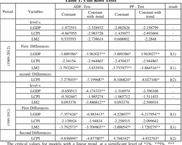
Results of ADF [17] and Phillips-Peron unit root tests [18] (with trend and without trend) are presented in Table1.Table shows these results for all series in levels, first and second differences for two sample periods. The null hypothesis of these tests is that series have a unit root or are non-stationary (table 1).
differencing respectively. Table 1 also shows that the unit root tests for those series in sub-sample period (1989-2012) has the same results as total period. The variable are integrated of order one I (1), two I (1), and two I (2) respectively.
Table 1: Unit Root Tests
Period Variables
ADF- Test PP - Test result Constant with trend Constant Constant Constant with trend level s:
LGDP -1.672551 -2.328932 -2.002826 -2.158799 - LCPI -0.867955 -2.983728 -1.435077 -2.493604 - LM2 0.535593 -2.738614 0.668802 -2.2848 -
(1
9
6
9
-2
0
1
2
) First Differences:
LGDP -3.889386* -3.963027** -3.889386* 3.963027** I(1) LCPI -2.54154 -2.944867 -2.470437 -2.944867 - LM2 -3.793282** -3.833976 -3.757977** -3.884516** I(1) second Differences:
LCPI -7.275035* -7.199687* -8.106824* -8.027160* I(2)
level s: -
LGDP -0.650513 -4.174333** -1.316974 -2.396168 - LCPI -0.392667 -1.985274 -1.065712 -1.511453 - LM2 0.093376 -3.486812** 0.093376 -2.596914
(1989
-2012
). First Differences:
LGDP -7.357426* -6.883413* -4.228037* -4.217954** I(1) LCPI -2.138924 -1.94834 -2.258515 -2.099642 - LM2 -3.792573* -3.709803** -3.800547* -3.720279** I(1) Second Differences:
LCPI -4.836694* -4.877807* 4.768342* -4.832763* I(2)
The critical values for models with a linear trend, at a significant level of *1%, **5%, *** 10% are:
Period (1) -4.144584, -3.498692, -3.178578 respectively. Period (2)-4.39430-3.612199-3.243079 respectively.
The critical values for models without a linear trend at a significant level of 1%, 5%, and 10% are:
Period (1) 3.562669,2.91877,2.597285 respectively. Period (2) 3.737853, 2.991878, -2.635542 respectively.
5-2- Cointegration TESTS
of the dynamic system should be a vector error correction model (VECM) [16].
Since the results of the co-integration test often depend on the number of lags, we used some appropriate VAR lag order selection tests such as likelihood ratio (LR), Akaike Information Criterion (AIC), Schwartz information criterion (SC), the Hannan-Quinn Information criterion (HQ), and Final prediction error (FPE) and to determine the proper lag length. Results signify two lags as a suitable lag length for two periods (Table 2).
Table 2: VAR Lag Order Selection test
Period Lag Log L LR FPE AIC SC HQ
(1
9
6
9
-2
0
1
2
) 185.1914 536.2116 1.08e-07 -7.530059 -7.053023 -7.351359 213.7886 48.49091* 4.63e08* -8.38211* -7.54729* -8.06938*
220.4903 10.48962 5.19e-08 -8.282186 -7.089593 -7.835433
(1
9
8
9
-2
0
1
2
) 0 0.348481 NA 0.000258 0.252526 0.401743 0.28491 1 107.0364 172.7327 2.39E-08 -9.051081 -8.454211 -8.921545
2 134.9613 37.23321* 4.20e09* -10.85345* -9.808930* -10.62676*
Notes: * indicates lag order selected by the criterion.
5-2-1- Johansen’s Co integration Test
Table 3: Unrestricted Co-integration Rank Test (Trace) Period Null Eigenvalue Trace Statistic 5% critical value Prob **
(1 9 8 9 -2 0 1 2
) r=0* 0.780399 51.51769 29.79707 0
r≤1 0.435885 15.13505 15.49471 0.0566
r≤2 0.056473 1.395116 3.841466 0.2375
(1 9 6 9 -2 0 1 2
) r=0* 0.428798 34.88178 29.79707 0.0119
r≤1 0.138077 7.441201 15.49471 0.5269
r≤2 0.003267 0.160351 3.841466 0.6888
Notes:Trace test indicate 1 co integrating vector at 5% level 1 co integrating vector for two periods.
*denotes rejection of the hypothesis at %5 level. **MacKinnon-Haug-Michelis (1999) p-values
Table 4: Unrestricted Co integration Rank Test (Maximum Eigen value)
Period Null Eigenvalue Max-Eigen Statistic 5% critical value Prob**
(1 9 8 9 -2 0 1 2 )
r=0* 0.780399 36.38264 21.13162 0.0002
r≤1 0.435885 13.73993 14.2646 0.0604 r≤2 0.056473 1.395116 3.841466 0.2375
(1 9 6 9 -2 0 1 2
) r=0* 0.428798 27.44058 21.13162 0.0057
r≤1 0.138077 7.28085 14.2646 0.4565
r≤2 0.003267 0.160351 3.841466 0.6888
Max-eigenvalue test indicate 1 co integrating vectors at 5% level 1 co integrating vector for two periods.
*denotes rejection of the hypothesis at %5 level. **MacKinnon-Haug-Michelis (1999) p-values.
According to the results of Trace and Max-Eigen value test (tables 3& 4), the null hypothesis of having no co-integrating vector has rejected at the five percent significance level
,
suggesting that there exists one co-integrating vector and one long run relationship between money supply, price and output for two periods.least one of the variables must respond to the magnitude of the disequilibrium. Therefore a vector error correction model (VECM) should be applied as a correct specification of model.
5-3- VECM: Estimated Vectors
By applying a three-variable VECM model with one cointegrating vector, we have examined Granger causality among the variables. Absence of Granger –Causality for cointegrated variables requires the additional condition that speed of adjustment coefficient be equal to zero. Lagged error-correction term, however, is a short-term adjustment coefficient and represents the long-term imbalance in the dependent variable that is being corrected in each period.
It should be noted that the number of cointegrating vectors indicates that there is consequent number of residual series as error-correction terms (ECTs). This term is a short–run adjustment parameter or speed of adjustment in estimated vector error-correction model (VECM).Error-correction terms (ECTs), can be represented as exogenous variables in vector error-correction model (VECM). Absence of significant coefficients for lagged variables show that there is no short run causality between variables in long run ECM models. The larger the error-correction term is the grater the response of subsequent variable to the previous period’s deviation from long –run equilibrium. At the opposite extreme, very small values of this term for each variable imply that it is unresponsive to last period`s equilibrium error.
Table 5: Cointegration Relationship between Money, Price and Output in two Period
Variables Sub-Period (1989-2012) Total Period (1969-2012)
LGDP(-1) 1
-3.034863 -0.25647 [-11.8333]
LM2(-1)
-0.235433
1 -0.0085
[-27.7103]
LCPI(-1)
0.080222 -0.806191 -0.01297 -0.06062 [ 6.18540] [-13.2980]
c -10.30035 31.24169
ECTs -0.642754 -0.09671 (Error-correction
terms) -0.14914 -0.02839 [-4.30985] [-3.40624] Assumption: Linear trend in data .Standard errors in ( ) & t-statistics in [ ].
Source: Estimated VECM Models.
Results also show that error-correction term or speed of adjustment in second period is higher (-0.64), than the first period ones (-0.09), indicating faster short run adjustment to the long run equilibrium in this period. This important deference for sub-period, during which the substantial increasing of liquidity (m2) had been carried out by central bank of Iran, is a key point for analyzing relationship between these variables and finding leading variables in this package to adopt proper economic policies in Iran.
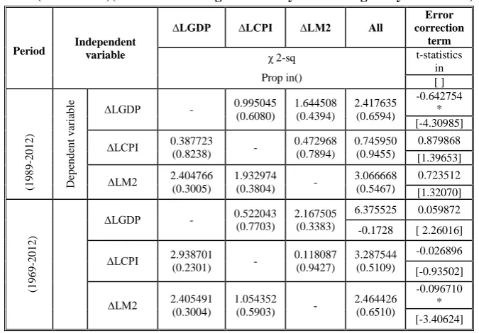
5-4- Granger Causality Tests Based on the VECM
Table 6: Granger Causality Tests Based on the VECM -Period (1989-2012) and Period (1969-2012 )(VEC and Granger Causality/Block Erogeneity Wald Test)
Period Independent variable
∆LGDP ∆LCPI ∆LM2 All
Error correction term χ 2-sq Prop in() t-statistics in [ ] (1 9 8 9 -2 0 1 2 ) D ep en d en t v ar ia b
le ∆LGDP - 0.995045 (0.6080) 1.644508 (0.4394) 2.417635 (0.6594) -0.642754 * [-4.30985] ∆LCPI 0.387723
(0.8238) -
0.472968 (0.7894) 0.745950 (0.9455) 0.879868 [1.39653] ∆LM2 2.404766
(0.3005)
1.932974 (0.3804) -
3.066668 (0.5467) 0.723512 [1.32070] (1 9 6 9 -2 0 1 2 )
∆LGDP - 0.522043 (0.7703)
2.167505 (0.3383)
6.375525 0.059872 -0.1728 [ 2.26016]
∆LCPI 2.938701 (0.2301) -
0.118087 (0.9427) 3.287544 (0.5109) -0.026896 [-0.93502]
∆LM2 2.405491 (0.3004)
1.054352 (0.5903) -
2.464426 (0.6510)
-0.096710 * [-3.40624]
Assumption:Linear trand in data .Source of coefficient and t-statistics: estimated VECM models (table 5).
Notes: A significant statistic implies that the independent variable Granger cause the dependent variable.
The χ 2 statistic tests the joint significance of each of the other lagged endogenous variables in the equation.
Results of estimated VECM model (table 5) signify that there is a long run causal relationship between money supply, output and price in two periods. But existence of long run relationships is against with causality in short time (table 6). Absence of short run Granger causality between variables (money, price and output) in 2 periods suggests that exogenous monetary policy shocks weren’t key sources of output and price variability for two periods in Iran.
5-5- Variance decomposition:
In period (1989-2012) at 9 year time horizon for GDP: GDP explains most of its own forecast error variance at first year (100%), this contribution decrease to 42% at year 5 and to 23% at year 9,contribution of CPI increase from 0% to 60% at the end.M2 explains 10% of GDP variance at year 3 , this contribution increase up t0 18% at year 5 and decrease to 15% at the end .For CPI: Only CPI explains most of the own forecast error variance at all years. Contribution of M2 from 0 at first to less than 1% ,and GDP from 0 up to 2% at the end of time horizon .For M2 : CPI explains 1.8% at first up to 14.7%at the end ,M2 explains 52.9% of the own forecast error variance at first but this Contribution decrease to 36.8% at the end year . Contribution of GDP to explain M2 forecast error variance increase from 45.2 to 51.4 at the year 7 and decrease to 48.3% at the end. Outcomes show that CPI has role of leading variable in this period (Table 7).
Table 7-Variance Decomposition period (1989-2012) Variance in: time horizon S.E LGDP LCPI LM2
LGDP
1 0.016773 100 0 0
3 0.032989 85.64679 3.994948 10.35826 5 0.048524 42.83762 38.51966 18.64272 7 0.063392 27.24777 56.51591 16.23633 9 0.073001 23.68443 60.88393 15.43164
LCPI
1 0.070858 0.042242 99.95776 0.000000 3 0.217267 0.454956 99.03792 0.507124 5 0.350002 1.628779 97.56076 0.810463 7 0.460348 2.196193 96.92273 0.881082 9 0.547784 2.326680 96.81611 0.857208
LM2
1 0.061612 45.20121 1.898516 52.90028 3 0.110098 46.23636 6.317588 47.44605 5 0.142058 50.48544 10.22807 39.28649 7 0.168400 51.41152 11.18556 37.40292 9 0.191677 49.00436 13.70149 37.29416 Cholesky Orering: LGDP LCPI LM2
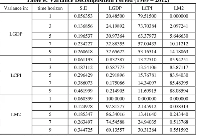
year (79.5%), this contribution decrease to 51.7% at year 9, contribution of CPI increase from 0% to 15.8% at the end.M2 explains 20.4% of GDP variance at first year, this contribution increase up t0 32.3% at the end .For CPI: Only CPI explains most of the own forecast error variance at all years of time in horizon (85.9-89%). Contribution of M2 to explain M2 forecast error variance only (0.8-0.11%) at all years, and Contribution of GDP decrease from 13.2% to 10.5% at the end of time horizon. Outcomes in this section confirm the last result that CPI has role of leading variable for this period (Table 8).
Table 8: Variance Decomposition Period (1969 – 2012) Variance in: time horizon S.E LGDP LCPI LM2
LGDP
1 0.056353 20.48500 79.51500 0.000000
3 0.136856 24.19892 73.70384 2.097241
5 0.196537 30.97364 63.37973 5.646630 7 0.234227 32.88355 57.00433 10.11212 9 0.260618 32.65622 53.16314 14.18063
LCPI
1 0.061193 0.832387 13.22510 85.94251 3 0.187112 0.587773 13.54106 85.87117 5 0.296429 0.291896 15.76781 83.94030 7 0.386073 0.175086 14.34097 85.48395 9 0.461999 0.214905 11.69915 88.08594
LM2
1 0.060399 100.0000 0.000000 0.000000 3 0.124978 97.81577 2.145912 0.038313 5 0.185347 86.34016 13.41640 0.243440 7 0.263497 74.54588 24.94035 0.513768 9 0.344725 69.13557 30.31284 0.551592 Cholesky Orering: LM2 LGDP LCPI
6- Conclusion
In this paper we reexamined the causal relationship between money, prices and output in Iran. We applied multivariate Granger-causality tests in a vector error correction model (VECM).The method applied here, highlights the fact that Granger causality may hold only in parts of the sample. Results were indicative of a co-integrated relationship between variables during the base sample period (1969 – 2012) and sub- sample (1989-2012).But direction of causality is deferent for period two. Although significant link between money, price and output was illustrated in co-integrated relationship at sub period (1989-2012), results of short run granger causality tests were contrast with them. Totally, the results of a three-variable vector error correction model (VECM) analysis was indicative for existence of one co-integrated relationship between money supply, price and real output in two period, but Granger-causality and variance decomposition tests didn’t confirm that money supply plays an important role in explaining real output fluctuations in Iran. This survey confirms the results of previous studies, which there was no causality link from money to output in Iran. This means monetary policy shocks weren’t sufficiently frequent and large to be statistically significant over sample period, or liquidity is not channeled toward production. It is very important to consider that long run relationship could come from correlation not causality. These results lead to other future surveys by using common variables that possibly will explain these relationships.Since the issue of money-output causality in Iran by applying econometrics estimation has been unresolved, so policymakers ought to adopt them with caution.
References
1- Erjavec, N. & B.Cota,” Macroeconomic Granger-Causal Dynamics in Croatia: Evidence Based on a Vector Error Modeling Analysis,”Ekonomski Pregled, 54: 139-156, 2003.
2- Freeman, Scott, “Money and Output: Correlation or Causality, “Economic Review, Federal Reserve Bank of Dallas, (3):1-7, 1992.
4- Abrishami, H,”Testing the long run neutrality of money based on the seasonal cointegration theory: the case of Iran,”Iranian Economic Review, 6: 5-23. 2002.
5- M. Kabir Hassan ,” Dynamic Linkages of Output, Money, Price and Exchange Rate and Central Bank Monetary Policy Management in Islamic Republic of Iran .Journal of Money and Economy,Vol.2. No.1, spring 2003.Journal of the Monetary and Banking Research Institute.
6- Bonato, L,”Money and Inflation in the Islamic Republic of Iran,” IMF Working Paper, Middle East and Central Asia Department, 2007.
7- Hayo, B,” Money-output Granger causality revisited: An empirical analysis of EU countries,” ZEI Working Paper 1998-08, University of Bonn, 1998.
8- Herwartz, H. & H.E.Reimers, ”Long-Run Links among Money, Prices, and Output: World-Wide Evidence, “Discussion paper, Economic Research Centre of the Deutsche Bundesbank, 2001.
9- Pesaran,H, ”Economic Trends and Macroeconomic Policies in Post-Revolutionary Iran, “Cambridge University, 1998.
10-Cortes, B. S. & D. Kong,” Regional Effects of Chinese Monetary Policy”, The International Journal of Economic Policy Studies, 2: 15-28, 2007.
11-Kiaee, H,” Monetary Policy in Islamic Economic Framework: Case of Islamic Republic of Iran”, Imam Sadiq University, Sep 2007. Online at: http://mpra.ub.uni-muenchen.de/4837/
12-Levent,K.& C.Saatçioğlu,” The search for co-integration between money, prices and income: low frequency evidence from the Turkish economy ,”Istanbul University Institute of Social Sciences, 2009.
13-(Online at http://mpra.ub.uni-muenchen.de/19557/)
14-Nwosa, P.I & I.O. Oseni”, Monetary Policy, Exchange Rate and Inflation Rate in Nigeria: A Co-integration and Multivariate Vector Error Correction Model Approach,” Research Journal of Finance and Accounting 15-ISSN 2222-1697 (Paper) ISSN 2222-2847.Vol 3, No 3, 2012.
16-Central Bank of Iran Website (www.cbi.ir)
17-Journal of Iran economics, Vol.XVI-No.174-Augest, 2013-IRR 35,000-ISSN 1562 3890
18-Enders, W, ”Applied econometric time series,” John Wiley & Sons, Inc., New York, 2000.
19-Dickey, D.A. and W.A, Fuller, “Distributions of the Estimators for Autoregressive Time Series with Unit Root, “Journal of the American Statistical Association, 74:427-431,1979.
20-Phillips, P.C.B. and P. Peron, “Testing for a Unit Root in Time Series Regression,” Biometrical, 75: 335-346, 1988.