Demonstrating The Use Of Vector Error
Correction Models Using Simulated Data
Carl B. McGowan, Jr., Norfolk State University, USA Izani Ibrahim, National University of Malaysia, Malaysia
ABSTRACT
In this paper, we demonstrate the use of time series analysis, including unit roots tests, Granger causality tests, cointergation tests and vector error correction models. We generate four time series using simulation such that the data has both a random component and a growth trend. The data are analyzed to demonstrate the use of time series analysis procedures.
Keywords: Time Series Analysis; Simulation; Unit Root Tests; Granger Causality; Cointegration; Vector Error Correction Models
INTRODUCTION
egressions between levels of variables may have high covariation because of persistence in the base levels of the variables rather than persistence in the changes in the values of the variables. Taking the first differences of the variables may eliminate, or at least reduce, the dependence between the variables. Gross national income from period to period is an integrated process, but the changes in GNI are not an integrated process. The first differences of GNI are an independent, identically distributed process which are only weakly dependent. An alternative transformation to differencing is to take the natural logarithm of the ratio of the two levels to generate the percentage rate of change which generates a continuously compounded rate of change.
STATIONARITY AND DICKEY-FULLER
Ordinary Least Squares regression requires that the time series being evaluated be stationary. Otherwise, OLS is no longer efficient, the standard errors are understated, and the OLS estimates are biased and inconsistent. Stationarity requires that the time series values for the mean, the standard deviation, and the covariance, be invariate over time1.
E(t-1) = E(t), i. e., t is constant over time, E(t-1) = E(t), i. e., t is constant over time, and
E(covt-1) = E(covt), i. e. the covariance of (xt, xt-1) is constant over time.
That is, the mean for any time (t-1) will equal the mean for any time (t), the standard deviation for any time (t-1) will equal the standard deviation for any time (t), and the covariance for any time (t-1) will equal the covariance for any time (t).
One method to test for stationarity is the unit root test of Dickey-Fuller (1979). To test for a unit root of a stochastic time series, the value of the random variable is regressed against lagged values of the same random variable
xt = + xt-1 + t [1]
where, xt is the value of the time series at time (t), is the intercept term, is the regression coefficient, xt-1 is the lagged value of the time series, and t is the residual. If is equal to one, then the process generating the time series is non-stationary. The null hypothesis is that H0: =1 and the alternative hypothesis is that is less than one, H1:
<1. The actual test is run after subtracting xt-1 from both sides of Equation [1]. The regression is
xt = *
+ *xt-1 + *
t [2]
where the (*) indicates the parameters from the regression adjusted by subtracting xt-1. The null hypothesis is that H0: *=0 and the alternative hypothesis is that is less than zero, H1:
* <0.
This model is only valid for AR(1) processes. If the underlying return generating process exhibits serial correlation of order greater than one, Augmented Dickey-Fuller tests must be used. Higher order terms are included in the regression
xt = * + *xt-1 + 1 xt-1 + 2 xt-2 +…. + n xt-n + *t [3]
where, the additional terms are derived from the higher order AR() terms. The null hypothesis is that H0: *=0 and the alternative hypothesis is that * is less than one, H1: *<0.
CO-INTEGRATION AND ENGLE-GRANGER
Co-integrated processes are random in the short-term but tend to move together in the long-term. Wooldridge (2003) shows that six-month Treasury bill rates and three-month Treasury bill rates are both unit root processes that are independent in the short-term but do not drift too far apart in the long-term. If either rate moves too far from equilibrium, either too high or too low, investors move money from the low (high) rate alternative to the high (low) rate alternative. This process will raise (lower) the rate in the low (high) rate market.
Engle and Granger (1987) show that if a linear combination of non-stationary time series is stationary, the time series is co-integrated. If two time series are integrated of order one, the time series resulting from adding the two is integrated of order one. If yt ~ I(1) and xt ~ I(1), then (yt + xt) ~ I(1). However, if a beta, , exits such that (yt - xt) ~ I(0), then yt and xt are said to be co-integrated. This co-integration equation reflects the long-term relationship between yt and xt.
If we can construct a linear combination of yt and xt such that the difference of the two variables has a unit root, the two variables are co-integrated and the regression coefficient is the co-integration parameter.
yt = 0 + 1xt + ut
If ut is I(0), then yt and xt are co-integrated. The model for testing for co-integration with a time trend includes a time variable.
yt = 0 + 2(t)+ 1xt + ut
If ut is I(0), then yt and xt are co-integrated.
ERROR CORRECTION MODELS
Error correction models are a class of models that provide insight into the long-term relationship between variables in terms of the “impact propensity, long run propensity, and lag distribution for y as a distributed lag in x.”2 The independent variable is x and the dependent variable is y. An error correction term is computed based on the past values of both x and y. If past values of y are over-estimated, future values will be moved back toward
2
equilibrium by the error correction factor. In the example of the six-month and three-month Treasury bill rates, the error correction term is computed from the difference of the one period lagged six-month rate and the two-period lagged three-month rate. Thus, if either of the two rates drift too far from the long-term rate, the error correction term shows the tendency of the rates to return to the long-term rate.
If two variables are cointegrated, we can construct a variable, st, which is I(0). The resulting error correction equation is
xt = * + *xt-1 + *yt + *yt-1 + *st-1 + *t [2]
where, st-1, equals (yt-1 - *
xt-1) and is the error correction term.
We can analyze the short-term effects of the relationship between the two variables. If the value of < 0, the error correction term serves to return the process to the long-run value. That is, if (yt-1 >
*
xt-1), the process was above the long-run value in the previous period and has been moved back by the error correction process.
GENERATING THE SIMULATED DATA
We use an Excel spreadsheet and the Excel function Rand() to generate four times series of numbers of 1,000 observations each. Rand() generates a number from zero to one. In order to create a random number series with a value of zero, the random number generated by Rand() is transformed into a zero value function by subtracting 0.50 from each Rand() value, Rand(*)=(Rand()-0.50). This random number generated by Rand() and transformed to a zero value number is used to create an Index value with the following equation:
Index(i,t) = Index(i,t-1) (1+Rand()(Return)+Trend)
Index(i,t) = Index(i,t-1) = 1.0000(1+0.0025+.005)
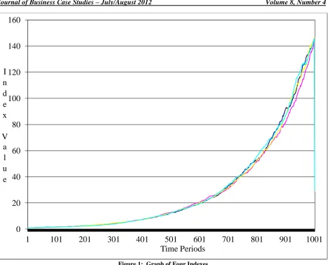
Index (i,t) is the index value for each period “t” that is calculated from the previous Index (i,t) value plus a randomly generated value with an expected value of zero plus the trend. The trend is a long-run trend added to the random index change in order to create both a random component of the Index plus a trend. Four Indexes are generated using this function with 1001 observations each.
Returns are calculated from each Index (i,t) using the natural logarithm function. Return(i,t) is the natural logarithm of the ratio of Index(i,t) divided by Index (i,t-1).
Return(i,t) = (Index(i,t)) / (Index (i,t-1))
Each return series has 1,000 observations that have both a random component and a trend component. The random component is the value of Rand(*)(Return) that is added to each previous Index (i,t) plus a trend.
ANALYSIS OF THE GENERATED RETURNS
Figure 1: Graph of Four Indexes Time Series Analysis Simulation
Figure 2: Summary Statistics for ROR01 Time Series Analysis Simulation
0
20
40
60
80
100
120
140
160
1
101
201
301
401
501
601
701
801
901
1001
I
n
d
e
x
V
a
l
u
e
Time Periods
0 20 40 60 80 100
-0.010 -0.005 0.000 0.005 0.010 0.015 0.020
S eries: R OR 01 S ample 1 1000 Observations 1000
Mean 0.004981
Median 0.005108
Maximum 0.019589
Minimum -0.009770
S td. D ev. 0.004965
S kewness -0.022106
K urtosis 2.893713
Jarque-B era 0.552149
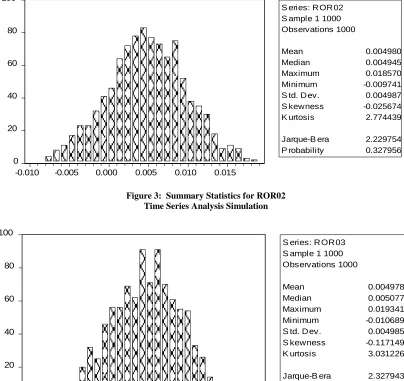
Figure 3: Summary Statistics for ROR02 Time Series Analysis Simulation
Figure 4: Summary Statistics for ROR04 Time Series Analysis Simulation
0 20 40 60 80 100
-0.010 -0.005 0.000 0.005 0.010 0.015
S eries: R OR 02 S ample 1 1000 Observations 1000
Mean 0.004980
Median 0.004945
Maximum 0.018570
Minimum -0.009741
S td. D ev. 0.004987
S kewness -0.025674
K urtosis 2.774439
Jarque-B era 2.229754
P robability 0.327956
0 20 40 60 80 100
-0.010 -0.005 0.000 0.005 0.010 0.015 0.020
S eries: R OR 03 S ample 1 1000 Observations 1000
Mean 0.004978
Median 0.005077
Maximum 0.019341
Minimum -0.010689
S td. D ev. 0.004985
S kewness -0.117149
K urtosis 3.031226
Jarque-B era 2.327943
Figure 5: Summary Statistics for ROR04 Time Series Analysis Simulation
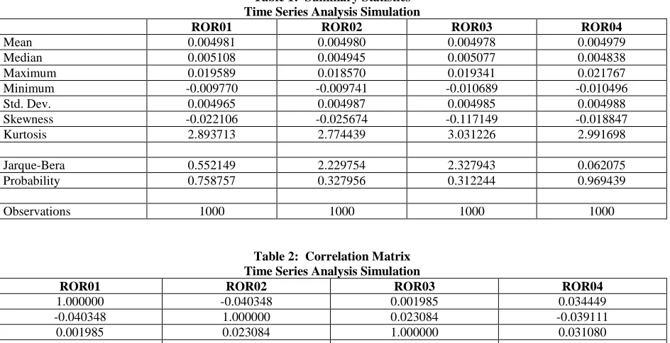
Table 2 contains the correlation matrix for the four Return(i,t) series. The four Return(i,t) series are constructed with a short-run random component and a long-run trend component. The correlation coefficients for the four Return(i,t) series reflect the short-run relationship between each of the Return(i,t) series. Thus, we see in Table 1 that the correlation coefficients for the four Return(i,t) series are all low and none are statistically significant.
Table 1: Summary Statistics Time Series Analysis Simulation
ROR01 ROR02 ROR03 ROR04
Mean 0.004981 0.004980 0.004978 0.004979
Median 0.005108 0.004945 0.005077 0.004838
Maximum 0.019589 0.018570 0.019341 0.021767
Minimum -0.009770 -0.009741 -0.010689 -0.010496
Std. Dev. 0.004965 0.004987 0.004985 0.004988
Skewness -0.022106 -0.025674 -0.117149 -0.018847
Kurtosis 2.893713 2.774439 3.031226 2.991698
Jarque-Bera 0.552149 2.229754 2.327943 0.062075
Probability 0.758757 0.327956 0.312244 0.969439
Observations 1000 1000 1000 1000
Table 2: Correlation Matrix Time Series Analysis Simulation
ROR01 ROR02 ROR03 ROR04
1.000000 -0.040348 0.001985 0.034449
-0.040348 1.000000 0.023084 -0.039111
0.001985 0.023084 1.000000 0.031080
0.034449 -0.039111 0.031080 1.000000
0 20 40 60 80 100
-0.010 -0.005 0.000 0.005 0.010 0.015 0.020
S eries: R OR 04 S ample 1 1000 Observations 1000
Mean 0.004979
Median 0.004838
Maximum 0.021767
Minimum -0.010496
S td. D ev. 0.004988
S kewness -0.018847
K urtosis 2.991698
Jarque-B era 0.062075
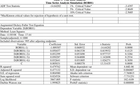
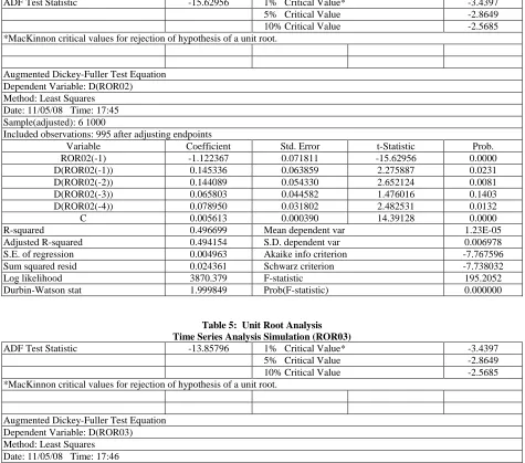
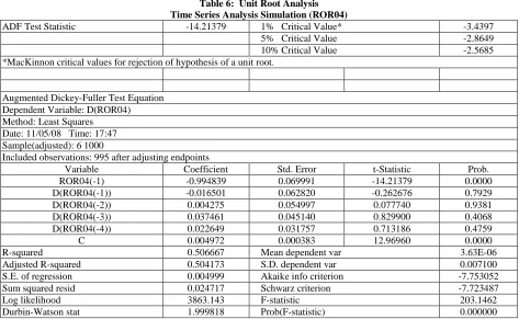
Generally, the first step in analyzing the relationships between time series is to determine if each Return(i,t) series has a unit root. The Augmented Dickey-Fuller test for a unit root is performed for each of the four Return(i,t) series and the empirical results are detailed in Table 3, Table 4, Table 5, and Table 6 for each simulated return series. For the Return(1,t) series, the ADF test statistic is 14.63 and the critical value for the ADF test statistic is -3.97 which indicates that Return(1,t) series does not have a unit root. None of the four lagged Return(1,t) series variable regression coefficients are statistically significant, but the intercept term is and equals 0.5014. The adjusted R2 for the regression is 0.4798 and the F-statistic is 152. These results reject the presence of a unit root. That is, Return(1,t) series does not have a unit root which is consistent with the method of creating the Return(i,t) series. The results for all four Return(i,t) series are similar to the results for Return(1,t) series.
Table 3: Unit Root Analysis Time Series Analysis Simulation (ROR01)
ADF Test Statistic -14.64202 1% Critical Value* -3.4397
5% Critical Value -2.8649
10% Critical Value -2.5685
*MacKinnon critical values for rejection of hypothesis of a unit root.
Augmented Dickey-Fuller Test Equation Dependent Variable: D(ROR01) Method: Least Squares
Date: 11/05/08 Time: 17:44 Sample(adjusted): 6 1000
Included observations: 995 after adjusting endpoints
Variable Coefficient Std. Error t-Statistic Prob.
ROR01(-1) -1.009307 0.068932 -14.64202 0.0000
D(ROR01(-1)) 0.050457 0.061538 0.819932 0.4125
D(ROR01(-2)) 0.052299 0.053490 0.977737 0.3284
D(ROR01(-3)) 0.050287 0.044008 1.142698 0.2534
D(ROR01(-4)) 0.032641 0.031805 1.026271 0.3050
C 0.005031 0.000378 13.31435 0.0000
R-squared 0.479762 Mean dependent var 4.66E-06
Adjusted R-squared 0.477132 S.D. dependent var 0.006887
S.E. of regression 0.004980 Akaike info criterion -7.760815
Sum squared resid 0.024526 Schwarz criterion -7.731251
Log likelihood 3867.005 F-statistic 182.4109
Table 4: Unit Root Analysis Time Series Analysis Simulation (ROR02)
ADF Test Statistic -15.62956 1% Critical Value* -3.4397
5% Critical Value -2.8649
10% Critical Value -2.5685
*MacKinnon critical values for rejection of hypothesis of a unit root.
Augmented Dickey-Fuller Test Equation Dependent Variable: D(ROR02) Method: Least Squares
Date: 11/05/08 Time: 17:45 Sample(adjusted): 6 1000
Included observations: 995 after adjusting endpoints
Variable Coefficient Std. Error t-Statistic Prob.
ROR02(-1) -1.122367 0.071811 -15.62956 0.0000
D(ROR02(-1)) 0.145336 0.063859 2.275887 0.0231
D(ROR02(-2)) 0.144089 0.054330 2.652124 0.0081
D(ROR02(-3)) 0.065803 0.044582 1.476016 0.1403
D(ROR02(-4)) 0.078950 0.031802 2.482531 0.0132
C 0.005613 0.000390 14.39128 0.0000
R-squared 0.496699 Mean dependent var 1.23E-05
Adjusted R-squared 0.494154 S.D. dependent var 0.006978
S.E. of regression 0.004963 Akaike info criterion -7.767596
Sum squared resid 0.024361 Schwarz criterion -7.738032
Log likelihood 3870.379 F-statistic 195.2052
Durbin-Watson stat 1.999849 Prob(F-statistic) 0.000000
Table 5: Unit Root Analysis Time Series Analysis Simulation (ROR03)
ADF Test Statistic -13.85796 1% Critical Value* -3.4397
5% Critical Value -2.8649
10% Critical Value -2.5685
*MacKinnon critical values for rejection of hypothesis of a unit root.
Augmented Dickey-Fuller Test Equation Dependent Variable: D(ROR03) Method: Least Squares
Date: 11/05/08 Time: 17:46 Sample(adjusted): 6 1000
Included observations: 995 after adjusting endpoints
Variable Coefficient Std. Error t-Statistic Prob.
ROR03(-1) -0.977154 0.070512 -13.85796 0.0000
D(ROR03(-1)) -0.030249 0.063229 -0.478401 0.6325
D(ROR03(-2)) -0.006233 0.054924 -0.113485 0.9097
D(ROR03(-3)) -0.007407 0.045141 -0.164077 0.8697
D(ROR03(-4)) -0.003669 0.031785 -0.115440 0.9081
C 0.004858 0.000385 12.63444 0.0000
R-squared 0.504057 Mean dependent var 3.28E-06
Adjusted R-squared 0.501550 S.D. dependent var 0.007089
S.E. of regression 0.005005 Akaike info criterion -7.750766
Sum squared resid 0.024774 Schwarz criterion -7.721202
Log likelihood 3862.006 F-statistic 201.0363
Table 6: Unit Root Analysis Time Series Analysis Simulation (ROR04)
ADF Test Statistic -14.21379 1% Critical Value* -3.4397
5% Critical Value -2.8649
10% Critical Value -2.5685
*MacKinnon critical values for rejection of hypothesis of a unit root.
Augmented Dickey-Fuller Test Equation Dependent Variable: D(ROR04) Method: Least Squares
Date: 11/05/08 Time: 17:47 Sample(adjusted): 6 1000
Included observations: 995 after adjusting endpoints
Variable Coefficient Std. Error t-Statistic Prob.
ROR04(-1) -0.994839 0.069991 -14.21379 0.0000
D(ROR04(-1)) -0.016501 0.062820 -0.262676 0.7929
D(ROR04(-2)) 0.004275 0.054997 0.077740 0.9381
D(ROR04(-3)) 0.037461 0.045140 0.829900 0.4068
D(ROR04(-4)) 0.022649 0.031757 0.713186 0.4759
C 0.004972 0.000383 12.96960 0.0000
R-squared 0.506667 Mean dependent var 3.63E-06
Adjusted R-squared 0.504173 S.D. dependent var 0.007100
S.E. of regression 0.004999 Akaike info criterion -7.753052
Sum squared resid 0.024717 Schwarz criterion -7.723487
Log likelihood 3863.143 F-statistic 203.1462
Durbin-Watson stat 1.999818 Prob(F-statistic) 0.000000
The next step in the time-series analysis process is to determine if the four Return(i,t) series Granger cause each other. Table 7 shows the Granger causality statistics for the four Return(i,t) series. There are six combinations of Granger causality between the four Return(i,t) series, such as a determination if Return(1,t) series Granger causes Return(2,t) series and vice versa. In all six cases, Granger causality is rejected, as would be expected since the short-run component for each of the four Return(i,t) series are randomly generated.
Table 7: Granger Causality Tests Time Series Analysis Simulation Date: 11/05/08 Time: 17:48
Sample: 1 1000 Lags: 2
Null Hypothesis: Obs F-Statistic Probability
ROR02 does not Granger Cause ROR01 998 1.34586 0.26079
ROR01 does not Granger Cause ROR02 0.62422 0.53589
ROR03 does not Granger Cause ROR01 998 2.82095 0.06003
ROR01 does not Granger Cause ROR03 0.88871 0.41151
ROR04 does not Granger Cause ROR01 998 0.65045 0.52203
ROR01 does not Granger Cause ROR04 2.51855 0.08109
ROR03 does not Granger Cause ROR02 998 0.43306 0.64865
ROR02 does not Granger Cause ROR03 2.51052 0.08174
ROR04 does not Granger Cause ROR02 998 0.39303 0.67511
ROR02 does not Granger Cause ROR04 0.19871 0.81982
ROR04 does not Granger Cause ROR03 998 2.85850 0.05783
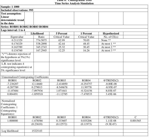
Once one has determined that the four Return(i,t) series are normally distributed with no statistically significant correlation, that the four Return(i,t) series are stationary with no unit roots, and that the four Return(i,t) series do not Granger cause each other, the four Return(i,t) series are tested for cointegration. Cointegration tests determine if the four Return(i,t) series have a long-run relationship that is not random as is the short-run relationship. Given that the four Return(i,t) series are constructed with an equal trend, we expect that the four Return(i,t) series will exhibit cointegration, which means that the four Return(i,t) series have a long-run relationship; i.e., the four Return(i,t) series follow the same long-run trend. Table 8 contains the results of the Johansen cointegration test. The test results indicate that there are four cointegrating equations at the 1% level of statistical significance as would be expected by the process by which in indices were constructed.
Table 8: Cointegration Tests Time Series Analysis Simulation Sample: 1 1000
Included observations: 995 Test assumption:
Linear
deterministic trend in the data
Series: ROR01 ROR02 ROR03 ROR04 Lags interval: 1 to 4
Likelihood 5 Percent 1 Percent Hypothesized Eigenvalue Ratio Critical Value Critical Value No. of CE(s)
0.211329 774.5075 62.99 70.05 None **
0.176329 538.2890 42.44 48.45 At most 1 **
0.163789 345.2743 25.32 30.45 At most 2 **
0.154760 167.2945 12.25 16.26 At most 3 **
*(**) denotes rejection of the hypothesis at 5%(1%) significance level L.R. test indicates 4 cointegrating equation(s) at 5% significance level
Unnormalized Cointegrating Coefficients:
ROR01 ROR02 ROR03 ROR04 @TREND(2)
-7.236207 12.14660 -2.414050 -0.254757 -8.00E-08
-0.287789 0.279013 -8.549678 11.99778 -8.95E-07
-11.87684 -7.897936 1.071641 -0.324156 8.03E-07
0.004491 -1.859518 -11.12785 -7.478533 3.45E-06
Normalized Cointegrating Coefficients: 1 Cointegrating Equation(s)
ROR01 ROR02 ROR03 ROR04 @TREND(2) C
1.000000 -1.678586 0.333607 0.035206 1.11E-08 0.001565
(0.23610) (0.12572) (0.11973) (9.3E-07)
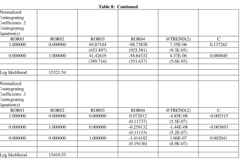
Table 8: Continued Normalized
Cointegrating Coefficients: 2 Cointegrating Equation(s)
ROR01 ROR02 ROR03 ROR04 @TREND(2) C
1.000000 0.000000 69.87104 -98.73838 7.35E-06 0.137262
(653.897) (925.581) (9.3E-05)
0.000000 1.000000 41.42619 -58.84332 4.37E-06 0.080840
(389.716) (551.637) (5.6E-05)
Log likelihood 15321.54
Normalized Cointegrating Coefficients: 3 Cointegrating Equation(s)
ROR01 ROR02 ROR03 ROR04 @TREND(2) C
1.000000 0.000000 0.000000 0.072012 -4.85E-08 -0.005315
(0.11737) (5.5E-07)
0.000000 1.000000 0.000000 -0.259132 -1.44E-08 -0.003693
(0.11115) (5.2E-07)
0.000000 0.000000 1.000000 -1.414182 1.06E-07 0.002041
(0.19130) (8.9E-07)
Log likelihood 15410.53
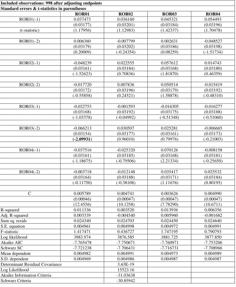
Table 9: Vector Error Correction Regression Time Series Analysis Simulation Sample(adjusted): 3 1000
Included observations: 998 after adjusting endpoints Standard errors & t-statistics in parentheses
ROR01 ROR02 ROR03 ROR04
ROR01(-1) 0.037473 0.036160 0.045321 0.054493
(0.03177) (0.03201) (0.03184) (0.03196)
(t-statistic) (1.17956) (1.12983) (1.42337) (1.70478)
ROR01(-2) 0.006360 -0.007799 0.002631 -0.048527
(0.03179) (0.03202) (0.03186) (0.03198)
(0.20009) (-0.24354) (0.08259) (-1.51734)
ROR02(-1) -0.048239 0.022555 0.057612 0.014743
(0.03161) (0.03184) (0.03168) (0.03180)
(-1.52623) (0.70836) (1.81870) (0.46359)
ROR02(-2) -0.017720 0.007836 0.050514 -0.015419
(0.03172) (0.03196) (0.03179) (0.03192)
(-0.55858) (0.24521) (1.58878) (-0.48310)
ROR03(-1) -0.032753 -0.001593 -0.016305 -0.016277
(0.03168) (0.03192) (0.03175) (0.03188)
(-1.03378) (-0.04992) (-0.51348) (-0.51060)
ROR03(-2) -0.066213 0.030507 0.025281 -0.006665
(0.03154) (0.03177) (0.03161) (0.03173)
(-2.09931) (0.96010) (0.79976) (-0.21003)
ROR04(-1) -0.037516 -0.025320 0.070126 -0.008158
(0.03161) (0.03185) (0.03168) (0.03181)
(-1.18675) (-0.79506) (2.21334) (-0.25650)
ROR04(-2) -0.003718 -0.012148 0.035417 0.025532
(0.03164) (0.03188) (0.03171) (0.03184)
(-0.11750) (-0.38108) (1.11676) (0.80195)
C 0.005789 0.004741 0.003626 0.004990
(0.00046) (0.00047) (0.00047) (0.00047)
(12.4556) (10.1258) (7.78290) (10.6711)
R-squared 0.011336 0.003520 0.013936 0.006356
Adj. R-squared 0.003339 -0.004540 0.005960 -0.001682
Sum sq. resids 0.024340 0.024703 0.024450 0.024640
S.E. equation 0.004961 0.004998 0.004972 0.004991
F-statistic 1.417471 0.436727 1.747195 0.790793
Log likelihood 3883.974 3876.585 3881.725 3877.850
Akaike AIC -7.765478 -7.750671 -7.760971 -7.753206
Schwarz SC -7.721238 -7.706431 -7.716731 -7.708966
Mean dependent 0.004982 0.004991 0.004973 0.004989
S.D. dependent 0.004969 0.004986 0.004987 0.004987
Determinant Residual Covariance 3.63E-19
Log Likelihood 15523.16
Akaike Information Criteria -31.03638
Table 10: VEC Regression Time Series Analysis Simulation Date: 11/05/08 Time: 17:52
Sample(adjusted): 4 1000
Included observations: 997 after adjusting endpoints Standard errors & t-statistics in parentheses
Cointegrating Eq: CointEq1
ROR01(-1) 1.000000
ROR02(-1) -3.107689
(0.56475) (-5.50280)
ROR03(-1) 0.912382
(0.23212) (3.93063)
ROR04(-1) -0.294429
(0.18021) (-1.63381)
@TREND(1) 2.80E-07
(1.7E-06) (0.16173)
C 0.007315
Error Correction: D(ROR01) D(ROR02) D(ROR03) D(ROR04)
CointEq1 -0.103659 0.292230 -0.065245 -0.004799
(0.01815) (0.01644) (0.01838) (0.01839)
(-5.71090) (17.7705) (-3.55066) (-0.26097)
D(ROR01(-1)) -0.564791 -0.168134 0.096734 0.085316
(0.03221) (0.02918) (0.03261) (0.03263)
(-17.5362) (-5.76207) (2.96677) (2.61473)
D(ROR01(-2)) -0.281775 -0.104444 0.048403 0.043913
(0.03050) (0.02763) (0.03088) (0.03090)
(-9.23802) (-3.77949) (1.56749) (1.42106)
D(ROR02(-1)) -0.271974 -0.024072 -0.085798 0.011477
(0.04767) (0.04319) (0.04826) (0.04829)
(-5.70549) (-0.55737) (-1.77788) (0.23765)
D(ROR02(-2)) -0.181455 0.029367 0.016240 0.004272
(0.03492) (0.03164) (0.03536) (0.03538)
(-5.19561) (0.92813) (0.45932) (0.12075)
D(ROR03(-1)) 0.045638 -0.193440 -0.647836 -0.023562
(0.03128) (0.02834) (0.03167) (0.03169)
(1.45908) (-6.82615) (-20.4587) (-0.74355)
D(ROR03(-2)) -0.016325 -0.079441 -0.303542 -0.023596
(0.02986) (0.02705) (0.03023) (0.03025)
Table 10: Continued
D(ROR04(-1)) -0.039442 0.050380 0.031532 -0.699384
(0.02978) (0.02698) (0.03015) (0.03017)
(-1.32425) (1.86700) (1.04573) (-23.1778)
D(ROR04(-2)) -0.017275 0.019816 0.028660 -0.347010
(0.02951) (0.02673) (0.02987) (0.02989)
(-0.58546) (0.74127) (0.95945) (-11.6084)
C 1.15E-05 8.67E-06 1.46E-06 1.04E-05
(0.00018) (0.00016) (0.00018) (0.00018)
(0.06462) (0.05373) (0.00809) (0.05745)
R-squared 0.338356 0.471541 0.359639 0.360589
Adj. R-squared 0.332323 0.466723 0.353800 0.354758
Sum sq. resids 0.031214 0.025621 0.031991 0.032037
S.E. equation 0.005624 0.005095 0.005693 0.005697
F-statistic 56.08207 97.85510 61.59097 61.84533
Log likelihood 3755.577 3854.005 3743.319 3742.601
Akaike AIC -7.513695 -7.711144 -7.489105 -7.487665
Schwarz SC -7.464500 -7.661949 -7.439910 -7.438470
Mean dependent 5.45E-06 9.04E-06 3.63E-07 4.64E-06
S.D. dependent 0.006882 0.006977 0.007082 0.007093
Determinant Residual Covariance 8.18E-19
Log Likelihood 15102.52
Akaike Information Criteria -30.20565
Schwarz Criteria -29.98427
THE VECTOR ERROR CORRECTION MODEL
Vector AutoRegression technique cannot be applied to the four Return(i,t) series because the four Return(i,t) series are cointegrated; that is, the four Return(i,t) series follow the same long-run trend, but the short-run trend is random. There are eight options for running the VEC model. The VEC model can be run with no trend in the VEC but with an intercept included or not. The VEC model can be run with a trend in the VEC and an intercept and/or a trend in the cointegration equation. The vector error correction equation uses lagged deviations for each of the four Return(i,t) series as independent variables for each of the four Return(i,t) series in a regression that also include lagged deviation variables for each of the four Return(i,t) series. Each set of VEC estimated regression includes the cointegrating equation plus a series of deviations from past changes in the four Return(i,t) series with up to two lags, unless more lags are specified. In addition, each VEC analysis can include a trend in the VEC and/or an intercept or a trend for each VEC. Table 10 contains the empirical results for the VEC model with a trend in the data and both an intercept and a trend in the error correction model. Given that the four Return(i,t) series are constructed with an intercept and a trend, the model with a trend in the data and a VEC model with both an intercept and a trend would seem to be most appropriate. The empirical results for this model show that the error correction equation is statistically significant but the trend is not statistically significant because the regression model accounts for the long-run trend effect across the four Return(i,t) series. Although the error correction variables are mostly statistically significant, the signs are random. This supports the hypothesis that cointegration is statistically significant but random in effect. The other three models provide similar results.
SUMMARY AND CONCLUSIONS
In this paper, we generated four Return(i,t) series using Excel that have both a random component and a trend component for each of the four Return(i,t) series. We applied a series of tests for time series analysis – correlation, normality, unit root, Granger causality, cointegration, and vector error correction regressions.
Return(i,t) series, which reflects the short-run random effect built into the four Return(i,t) series, no unit roots, and cointegration between the four Return(i,t) series, which Return(i,t) series is consistent with the method of constructing the four with a trend. Since the four Return(i,t) series are cointegrated by construction, a vector error correction model is appropriate for analysis of the long-run relationship between each of the four Return(i,t) series. The coinetegration equation is statistically significant as are the error correction variables, but in a random fashion with some of the regression coefficients being positive and some being negative.
In this paper, we show how to use the time series paradigm currently being used to conduct time series analysis. The basis of this analysis is the work in time series analysis done by noble laureate Engle and Granger. We demonstrate each of the steps designed to allow the researcher to determine if a relationship exists between two time series and to define the nature of that relationship.
AUTHOR INFORMATION
Carl B. McGowan, Jr., PhD, CFA is a Faculty Distinguished Professor and Professor of Finance at Norfolk State University, has a BA in International Relations (Syracuse), an MBA in Finance (Eastern Michigan), and a PhD in Business Administration (Finance) from Michigan State. From 2003 to 2004, he held the RHB Bank Distinguished Chair in Finance at the Universiti Kebangsaan Malaysia and has taught in Cost Rica, Malaysia, Moscow, Saudi Arabia, and The UAE. Professor McGowan has published in numerous journals including American Journal of Business Education, Applied Financial Economics, Decision Science, Financial Practice and Education, The Financial Review, International Business and Economics Research Journal, The International Review of Financial Analysis, The Journal of Applied Business Research, The Journal of Business Case Studies, The Journal of Diversity Management, The Journal of Real Estate Research, Managerial Finance, Managing Global Transitions, The Southwestern Economic Review, and Urban Studies. E-mail: [email protected]. Corresponding author.
Izani Ibrahim, PhD, is a Professor of Econometrics and Corporate Finance at the Graduate School of Business, National University of Malaysia. He received his B.Sc. (Actuarial Science) in 1985, from Pennsylvania State University, USA, and both his M.Sc. (Actuarial Science), in 1992 and Ph.D. (Finance), in 1996 from University of Nebraska, USA. Professor Izani has been giving lectures in quantitative methods at graduate level and to public and private sectors especially in Multivariate Analysis and Econometrics. His research interest in the finance area includes topics on corporate finance, derivatives and investment. Professor Izani has published in Capital Market Review, International Business & Economics Research Journal, International Research Journal, Journal of Current Research in Global Business, Journal of International Trade and Economic Development, Journal Analisis, and Journal Pengurusan. E-mail: [email protected]
REFERENCES
1. Dickey, D.A. and W.A. Fuller (1979) “Distribution of the Estimators for Autoregressive Time Series with a Unit Root,” Journal of the American Statistical Association, 74, 427–431.
2. Engle, Robert F. and C.W.J. Granger (1987) “Co-integration and Error Correction: Representation, Estimation, and Testing,” Econometrica 55, 251–276.
3. Jarque, C. and A. Bera (1980) "Efficient Tests for Normality, Homoskedasticity, and Serial Independence of Regression Residuals," Economics Letters, 6, 255–259.
4. Johansen, Soren (1991) “Estimation and Hypothesis Testing of Cointegration Vectors in Gaussian Vector Autoregressive Models,” Econometrica, 59, 1551–1580.
5. Johansen, Soren and Katarina Juselius (1990) “Maximum Likelihood Estimation and Inferences on Cointegration—with applications to the demand for money,” Oxford Bulletin of Economics and Statistics, 52, 169–210.