University of New Hampshire
University of New Hampshire Scholars' Repository
Master's Theses and Capstones Student Scholarship
Spring 2019
CONTROL STRATEGY OF MULTIROTOR
PLATFORM UNDER NOMINAL AND FAULT
CONDITIONS USING A DUAL-LOOP
CONTROL SCHEME USED FOR
EARTH-BASED SPACECRAFT CONTROL TESTING
Sital Khatiwada
University of New Hampshire, Durham
Follow this and additional works at:https://scholars.unh.edu/thesis
This Thesis is brought to you for free and open access by the Student Scholarship at University of New Hampshire Scholars' Repository. It has been accepted for inclusion in Master's Theses and Capstones by an authorized administrator of University of New Hampshire Scholars' Repository. For more information, please [email protected].
Recommended Citation
Khatiwada, Sital, "CONTROL STRATEGY OF MULTIROTOR PLATFORM UNDER NOMINAL AND FAULT CONDITIONS USING A DUAL-LOOP CONTROL SCHEME USED FOR EARTH-BASED SPACECRAFT CONTROL TESTING" (2019). Master's Theses and Capstones. 1276.
CONTROL STRATEGY OF MULTIROTOR PLATFORM UNDER NOMINAL AND FAULT CONDITIONS USING A DUAL-LOOP CONTROL SCHEME USED FOR EARTH-BASED SPACECRAFT CONTROL TESTING
BY
SITAL KHATIWADA
BS, University of New Hampshire, 2016
THESIS
Submitted to the University of New Hampshire
in Partial Fulfillment of
the Requirements for the Degree of
Master of Science
in
Mechanical Engineering
ALL RIGHTS RESERVED
c 2019
This thesis has been examined and approved in partial fulfillment of the requirements for
the degree of Master of Science in Mechanical Engineering by:
Thesis Director, Dr. May-Win L. Thein, Associate
Pro-fessor of Mechanical Engineering
Dr. Barry Fussell, Professor of Mechanical Engineering
Dr. Se Young Yoon, Assistant Professor of Electrical
Engineering
On 05/14/2019
Original approval signatures are on file with the University of New Hampshire Graduate
ACKNOWLEDGEMENTS
I would like to first thank the many individuals who helped me get to this far, either directly
or indirectly. Whether they were extended interactions or brief, yet inspired encounters, my
thanks go out to the many people who inspired me to reach where I am today.
To Prof. May-Win Thein, for bringing me under her wing when I first arrived at UNH.
I would not be where I am today without your guidance and encouragement.
To Prof. Barry Fussell, for his patience in teaching and ability to challenge students to
become better. I would also like to express my thanks for serving in my committee.
To Prof. Se Young Yoon, for challenging me in your courses and being available for any
inquiries. I would also like to express my thanks for serving in my committee.
To my Mom and Dad, who have sacrificed so much to give me this opportunity. I hope
I can make it up to them one day.
To my brother Arjun, who has always provided advice and encouraged me.
To Makenzie, who always managed to keep my head up when things were not going well.
To my lab mates, and my fellow graduate students. I did it, so can you.
Finally, to the UNH QuadSat Team, who assisted with the development of the
TABLE OF CONTENTS
ACKNOWLEDGEMENTS v
LIST OF TABLES x
LIST OF FIGURES xii
ABSTRACT xviii
1 INTRODUCTION 1
1.1 Quadrotors as Earth-based Satellite Test Platforms . . . 1
1.2 Quadrotor Control and Fault-Tolerance . . . 2
1.2.1 Control Gain Tuning . . . 4
1.3 Introduction to Quadrotor Platforms . . . 4
1.4 Quadcopter Classification . . . 5
1.5 Brief History of Quadcopters . . . 5
1.6 Multirotor Hardware . . . 7
1.7 Objective . . . 9
1.8 Thesis Overview and Structure . . . 10
2 DYNAMIC MODEL OF A QUADROTOR 11 2.1 Coordinate System, Reference Frames, and Rotation Matrices . . . 12
2.2 System Inputs . . . 13
2.4 Rotational Dynamics of Quadrotor . . . 22
2.5 Translational Dynamics of Quadrotor . . . 23
2.6 Unmodeled Dynamics of the Quadrotor System . . . 24
2.7 Unified Dynamic Model . . . 28
3 QUADROTOR CONTROL SCHEME 30 3.1 Nominal Control Method . . . 31
3.1.1 Inner Loop Attitude Control Scheme . . . 31
3.1.2 Outer Loop Position Control Scheme . . . 33
3.2 Fault Tolerant Control for Motor Performance Loss . . . 34
3.3 Sliding Mode Control Reachability Condition . . . 35
3.3.1 Nominal SMC Stability and Gain Range . . . 36
3.3.2 Compensated SMC Stability . . . 37
3.4 Controller Tuning through Particle Swarm Optimization Method . . . 39
3.4.1 PSO Algorithm Initialization . . . 40
3.4.2 Optimization Variables, Cost Function, and Gain Ranges . . . 42
4 PSO TUNING PROCESS AND RESULTS 45 4.1 PSO Tuning Results . . . 45
4.1.1 Attitude SMC Tuning . . . 45
4.1.2 Position PID Tuning . . . 53
4.2 Nominal Control Scheme Results . . . 61
4.3 Fault Tolerant Control Scheme Results . . . 63
5 EXPERIMENTAL DESIGN OF QUADROTOR PLATFORM 68 5.1 Flight Controller Components . . . 69
5.1.1 Microcontroller . . . 69
5.2 Rotor and Fault Diagnostics Systems . . . 74
5.2.1 Actuator System . . . 74
5.2.2 Fault Detection Mechanism . . . 75
5.3 Generation of Desired Pulse Width from Control Scheme Output . . . 79
5.4 Data Acquisition Module . . . 83
5.5 Experimental Quadrotor Control System Schematic . . . 84
5.6 Application of Control Scheme . . . 84
6 EXPERIMENTAL RESULTS 89 6.1 Rotor Compatibility and Ease of Control Testing . . . 89
6.2 SMC Attitude Control and Fault Tolerance Testing . . . 90
7 PROOF OF CONCEPT APPLICATION: HOHMANN TRANSFER 104 7.1 Brief Introduction to Hohmann Transfer Orbit . . . 104
7.2 Mimicked Hohmann Transfer using Quadrotor Platforms . . . 106
7.3 Feasability and Future of Multirotors as Satellite Test Platforms . . . 108
8 FUTURE STUDY: NONLINEAR STATE OBSERVER DESIGN FOR SENSOR FAULT 110 8.1 Linear Luenberger Observer . . . 111
8.2 Design of a Thau Observer . . . 112
9 CONCLUSION 121 9.1 Research Summary . . . 121
9.2 Future Works . . . 123
LIST OF REFERENCES 125
A AERODYNAMIC FORCE AND MOMENT CONSTANT
B GAIN TUNING COST PROPAGATIONS 131
LIST OF TABLES
2.1 Drag Upper Bound Calculation Parameters . . . 26
2.2 Calculated CD and Fd Upper Bound for x, y and z through Flow Simulation 26 2.3 Calculated Moment Upper Bound for φ, θ and ψ through Flow Simulation . 28 2.4 Uncertainty Upper bound . . . 28
2.5 System Parameters . . . 29
3.1 Sliding Mode Controller Stable Gain Range . . . 38
4.1 Tuned Attitude SMC Gains . . . 52
4.2 Initial PID Control Gains (Not tuned) . . . 53
4.3 Initial gain range for position PID controller . . . 57
4.4 PSO Tuned PID Gains . . . 59
4.5 Refined gain range for position PID controller . . . 59
4.6 Refined PSO Tuned PID Gains . . . 60
4.7 Tuned Control Scheme Gains . . . 61
4.8 Fault scenarios and max. tolerable fault magnitudes for different control schemes 64 5.1 Comparison of microcontroller candidates . . . 70
A.1 25lbf Load Cell Calibration for Kf . . . 129
A.2 25lbf Load Cell Calibration for Km . . . 130
A.3 25lbf Load Cell Calibration for Kf and Km . . . 130
LIST OF FIGURES
1.1 UNH TableSat 1C Experimental Test Bed [1] . . . 2
1.2 Rotor configurations for pitch/roll (left), yaw (center), heave/hover (right) [2] 4 1.3 UAV Classification Scheme . . . 6
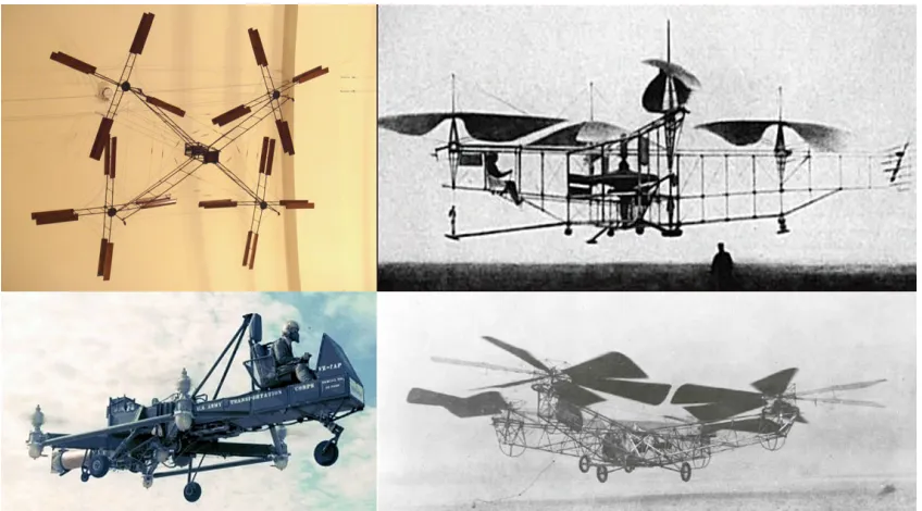
1.4 Early Multirotor Systems (counterclockwise from top left): Louis Charles Breguet’s aircraft, Oehmichen No.2, de Bothezat helicopter, Curtiss-Wright VZ-7 . . . 7
1.5 Modern UAVs . . . 7
2.1 Quadrotor Model . . . 11
2.2 Load Cell Calibration Curve forKf Identification . . . 18
2.3 Load Cell Calibration Curve forKm Identification . . . 18
2.4 Reflective tape applied to quadrotor propeller . . . 19
2.5 Quadrotor mounted onto the rotating fixture with the load cell . . . 19
2.6 Kf test experimental setup . . . 20
2.7 Km test experimental setup . . . 20
2.8 Rotor Speed/System Input relationship for Kf determination . . . 21
2.9 Rotor Speed/System Input relationship for Km determination . . . 21
2.10 SolidWorks Flow Simulation Velocity Profile during Vertical Ascent . . . 26
2.11 Cantilever Beam Representation of Quadrotor Arm . . . 27
2.12 SolidWorks Flow Simulation Velocity Profile during Crosswind . . . 28
3.2 PSO weight function behavior with intersection points for Kc = 100 . . . 41
4.1 SMC Tuned Gains for ranges shown in Table 3.1 and weights of Equations
(4.1) and (4.2) [Kc= 100,Ipi= 30] . . . 46
4.2 Propagation of cost for ranges shown in Table 3.1 and weights of Equations
(4.1) and (4.2) [Kc= 100,Ip= 30] . . . 46
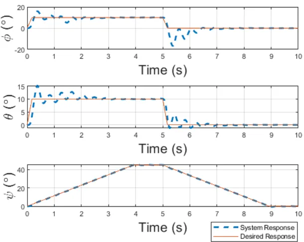
4.3 Response of SMC attitude control with tuned gains for ramp inputs . . . 48
4.4 Error of SMC attitude control with tuned gains for ramp inputs . . . 48
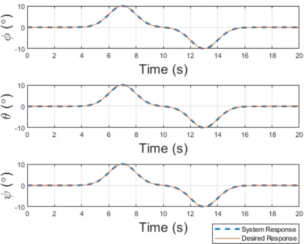
4.5 Response of SMC attitude control with tuned gains for Gaussian inputs . . . 49
4.6 Error of SMC attitude control with tuned gains for Gaussian inputs . . . 49
4.7 SMC-1 Tuned Gains for ranges shown in Table 3.1 and weights of Equations
(4.1) and (4.2) [Kc= 10, Ip= 100] . . . 50
4.8 SMC-2 Tuned Gains for ranges shown in Table 3.1 and weights of Equations
(4.1) and (4.2) [Kc= 10, Ip= 100] . . . 51
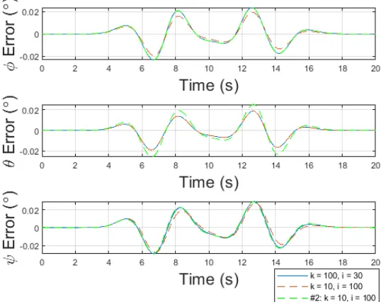
4.9 Comparative error between gain sets obtained through PSO for ramp input . 52
4.10 Comparative error between gain sets obtained through PSO for Gaussian input 52
4.11 Initial combined SMC/PID control scheme sinusoidal input using gains in
Table 4.1 and 4.2 . . . 55
4.12 Initial combined SMC/PID control scheme sinusoidal input ramp input
posi-tion error using gains in Table 4.1 and 4.2 . . . 55
4.13 Initial combined SMC/PID control scheme ramp input using gains in Table
4.1 and 4.2 . . . 56
4.14 Initial combined SMC/PID control scheme position error using gains in Table
4.1 and 4.2 . . . 56
4.15 PID Tuned Gains for ranges shown in Table 4.3 and weights of Equations (4.6)
and (4.7) [Kc= 10,Ip= 100]. Top Row: PID gains for x-position, Middle Row:
4.16 PID Propagation of cost for ranges shown in Table 4.3 and weights of
Equa-tions (4.6) and (4.7) [Kc= 10, Ip= 100]. The lowest cost value is marked . . 58
4.17 Position error comparison between initial, tuned, and refined PID controller gain sets for flight path in Equation (4.4) . . . 60
4.18 Position error comparison between initial, tuned, and refined PID controller gain sets for flight path in Equation (4.5) . . . 61
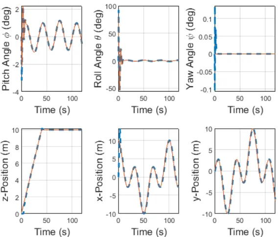
4.19 Quadrotor response to flight path in Equation (4.4) using SMC/PID control scheme . . . 62
4.20 Quadrotor flight path under nominal conditions . . . 62
4.21 Quadrotor response to flight path in Equation (4.4) using SMC-I/PID control scheme . . . 65
4.22 Quadrotor flight path under nominal conditions for SMC-I/PID control scheme 65 4.23 Quadrotor flight path under faulty conditions for SMC-I/PID control scheme 66 5.1 YMFC Auto Leveling Quadrotor Schematic [3] . . . 68
5.2 Completed quadrotor platform with radio controller . . . 69
5.3 Teensy 3.5 [4] . . . 71
5.4 Orientation of Axes of Sensitivity and Polarity of Rotation [5] . . . 71
5.6 Base components of the Marvelmind Indoor Navigation System [6] . . . 73
5.7 BLDC utilized on board the quadrotor platform [7] . . . 74
5.8 IR Optical Sensor [8] . . . 77
5.9 Integrated circuit for IR . . . 77
5.10 Detailed circuit layout for the motor speed sensor platform . . . 78
5.11 Response speed of the IR Sensor Suite (τ = 0.436s) . . . 79
5.12 Rotor speed and pulse signal mapped with a fifth-order polynomial fit for 10×4.5in propellers . . . 80
5.14 Propellers utilized for quadrotor flight: (in descending order) 10×4.5in, 9×4.7in,
and 8×4.5in . . . 82
5.15 HC-06 Bluetooth Module [9] . . . 83
5.16 Bluetooth module mounted on board the quadrotor platform . . . 83
5.17 Experimental Platform Control System Schematic . . . 84
5.18 MotionCal Calibration . . . 85
5.19 Mobile beacon mounted on quadrotor platform . . . 86
5.20 IR sensor module mounted on quadrotor arm for motor speed determination 88 6.1 Attitude Response of Quadrotor Platform with 10×4.5in Propeller . . . 90
6.2 System Input of Quadrotor Platform with 10×4.5in Propeller . . . 91
6.3 Attitude Response of Quadrotor Platform with 9×4.7in Propeller . . . 91
6.4 System Input of Quadrotor Platform with 9×4.7in Propeller . . . 92
6.5 Attitude Response of Quadrotor Platform with 8×4.5in Propeller . . . 93
6.6 System Input of Quadrotor Platform with 8×4.5in Propeller . . . 93
6.7 Nominal SMC Attitude Response of Quadrotor Platform . . . 94
6.8 Nominal SMC Attitude System Input . . . 94
6.9 Nominal SMC Nominal System Rotor Speed . . . 95
6.10 Quadrotor Platform Test Area . . . 95
6.11 Disturbance signal injected to Motor 1 mid flight . . . 96
6.12 Single Fault SMC+FTC Attitude Response for Fault Mid Flight . . . 96
6.13 Single Fault SMC+FTC System Input for Fault Mid Flight . . . 97
6.14 Single Fault SMC+FTC Attitude Response of Quadrotor Platform . . . 98
6.15 Single Fault SMC+FTC Attitude System Input . . . 98
6.16 Single Fault SMC+FTC System Rotor Speed . . . 99
6.17 Single Fault SMC+FTC System Rotor Speed . . . 99
6.20 Twin Fault SMC+FTC System Rotor Speed . . . 101
6.21 Twin Fault SMC+FTC System Rotor Speed . . . 102
6.22 Lowered chattering observed by lowering discontinuous control gains . . . 103
7.1 Transition from a lower orbit (1) to a higher orbit (3), with a Hohmann transfer (2) [10] . . . 105
7.2 Simulated Path for mimicked Hohmann transfer using quadrotor platform dynamics . . . 106
7.3 Velocity profiles of x and y components of the quadrotor during simulated “orbital transfer” . . . 107
7.4 ∆v profile of the quadrotor platform during simulated “orbital transfer” . . . 107
7.5 Omni-directional multirotor platform, referred to as an Omnicopter [11] . . . 109
8.1 Nominal Case Estimation Results . . . 115
8.2 Estimation Error for System Response in Figure 8.1 . . . 115
8.3 Nominal Case Estimation Results Using Gains in Equation (8.12) . . . 117
8.4 Nominal Case Estimation Error . . . 117
8.5 Nominal Case Estimation Error with Noise . . . 119
8.6 Nomincal Case Estimation Error with Noise . . . 119
8.7 Band-Limited White Noise Profile . . . 120
B.1 SMC-1 Propagation of cost for ranges shown in Table 3.1 and weights of Equations (4.1) and (4.2) [Kc= 10,Ip= 100] . . . 131
B.2 SMC-2 Propagation of cost for ranges shown in Table 3.1 and weights of Equations (4.1) and (4.2) [Kc= 10,Ip= 100] . . . 132
B.3 Tuned combined SMC/PID control scheme response using gains in Table 4.1 and 4.4 and flight path in Equation (4.4) . . . 132
B.5 Tuned combined SMC/PID control scheme response using gains in Table 4.1
and 4.4 and flight path in Equation (4.5) . . . 133
B.6 Tuned combined SMC/PID control scheme error using gains in Table 4.1 and
4.4 and flight path in Equation (4.5) . . . 134
B.7 Refined PID Tuned Gains for ranges shown in Table 4.5 and weights of
Equa-tions (4.6) and (4.7) [Kc= 10, Ip= 100] . . . 134
B.8 Refined PID Propagation of cost for ranges shown in Table 4.5 and weights
of Equations (4.6) and (4.7) [Kc= 10,Ip= 100] . . . 135
B.9 Tuned combined SMC/PID control scheme response using gains in Table 4.1
and 4.6 and flight path in Equation (4.4) . . . 135
B.10 Tuned combined SMC/PID control scheme error using gains in Table 4.1 and
4.6 and flight path in Equation (4.4) . . . 136
B.11 Tuned combined SMC/PID control scheme response using gains in Table 4.1
and 4.6 and flight path in Equation (4.5) . . . 136
B.12 Tuned combined SMC/PID control scheme error using gains in Table 4.1 and
ABSTRACT
CONTROL STRATEGY OF MULTIROTOR PLATFORM UNDER NOMINAL AND
FAULT CONDITIONS USING A DUAL-LOOP CONTROL SCHEME USED FOR
EARTH-BASED SPACECRAFT CONTROL TESTING
by
Sital Khatiwada
University of New Hampshire, May, 2019
Over the last decade, autonomous Unmanned Aerial Vehicles (UAVs) have seen
in-creased usage in industrial, defense, research, and academic applications. Specific attention
is given to multirotor platforms due to their high maneuverability, utility, and
accessibil-ity. As such, multirotors are often utilized in a variety of operating conditions such as
populated areas, hazardous environments, inclement weather, etc. In this study, the
effec-tiveness of multirotor platforms, specifically quadrotors, to behave as Earth-based satellite
test platforms is discussed. Additionally, due to concerns over system operations under such
circumstances, it becomes critical that multirotors are capable of operation despite
experi-encing undesired conditions and collisions which make the platform susceptible to on-board
hardware faults. Without countermeasures to account for such faults, specifically actuator
faults, a multirotors will experience catastrophic failure.
In this thesis, a control strategy for a quadrotor under nominal and fault conditions is
dual-loop SMC/PID control scheme is proposed to control the attitude and position states
of the nominal system. Actuator faults on-board the quadrotor are interpreted as motor
performance losses, specifically loss in rotor speeds. To control a faulty system, an additive
control scheme is implemented in conjunction with the nominal scheme.
The quadrotor platform is developed via analysis of the various subcomponents. In
addi-tion, various physical parameters of the quadrotor are determined experimentally. Simulated
and experimental testing showed promising results, and provide encouragement for further
CHAPTER 1 INTRODUCTION
1.1 Quadrotors as Earth-based Satellite Test Platforms
With regards to the University of New Hampshire Advanced Controls Lab (ACL), use of
quadrotor platforms to test satellite control algorithms have been considered in the past.
Previous iterations of research into development of Earth-based satellite test platform have
utilized a frictionless environment, specifically UNH TableSat. The purpose of TableSat was
to supplement NASA’s Magnetospheric Multiscale (MMS) mission, specifically to test and
analyze effects of the instrumentation booms on the satellite dynamics [1] [12]. While
Ta-bleSat was successful in studying the boom dynamics of the MMS platforms, the constraints
placed on the degrees of freedom, which included spin and limited nutation, along with a
specific application prohibits its use as a general satellite test platform. Comparable results
are found in similar platforms as well, as they cannot test 6-DOF systems [13] [14]. Thus,
the validity of a quadrotor platform is considered as an Earth-based satellite test bed.
In addition, the application of a formation of quadrotors to test satellite constellation
algorithms is considered. Past external research shows limited work in terms of utilizing
quadrotor platforms as spacecraft research test beds. Prior work performed by the author
has studied the feasibility of a quadrotor to mimic satellite systems through the use of an
in-house manufactured quadrotor and stereo vision motion tracking system [15].
Current research at the ACL seeks to develop quadrotors as low-cost economical
alterna-tive that can be used as Earth-based satellite test platforms for dynamics and control studies.
Figure 1.1: UNH TableSat 1C Experimental Test Bed [1]
of omni-directional control, due to the highly coupled nature of the quadrotor platform’s
states. A potential solution is to increase the number of actuators on-board the quadrotor,
allowing for independent state control, improved maneuverability, and added redundancies
in case of actuator faults. The long-term objective of the ACL is to eventually develop an
array of omnicopters, which are closest in likeness to satellite dynamics [11]. However, the
use of quadcopters as a current, viable Earth-based test platform is the focus of this research.
1.2 Quadrotor Control and Fault-Tolerance
Over the last decade, autonomous UAVs have seen increased usage in industrial, defense,
research, and academic applications. Specific attention is given to quadrotor platforms due to
their high maneuverability, utility, and accessibility. As such, quadrotors are often utilized in
a variety of operating conditions such as populated areas, hazardous environments, inclement
weather, etc. Due to concerns over system operations under such circumstances, it becomes
critical that quadrotors are capable of operation despite experiencing undesired conditions
and collisions which make the platform susceptible to on-board hardware faults. Without
settings, a failure can lead to damage or loss of the platform to injuries being inflicted on
any persons in the area. Therefore, to prevent such incidents, a reliable control scheme is
necessary.
Previous studies into quadrotor nominal and fault-tolerant control has included a myriad
of techniques. Linear control methods work well under nominal conditions, however
ensur-ing fault tolerance usually require a specific fault configuration or additional redundancies to
properly compensate for large scale faults, such as coaxial propeller systems [16] [17].
Non-linear control methods are more common and can provide added robustness to the system
under nominal and fault conditions. Control strategies such as Sliding Mode Control (SMC),
Backstepping, H∞ Control, or Model Predictive Adaptive Control (MPAC) are attractive
prospects for control techniques [18] [19] [20] [21] [22]. Such methods are used in conjunction
with fault detection methods using sensor arrays and observers. Observers are used to
iden-tify and reconstruct faults, such that the appropriate control can be applied to stabilize the
system [18] [23] [24]. Control reconfiguration techniques can also be used, which restructures
the control loop based on the diagnosed fault [25]. Pulse-Width Modulation (PWM) signals
can be studied to determine fault conditions of motors [24].
The type and magnitude of fault is critical towards leading the system towards
stabiliza-tion. Motor performance losses that do not cause complete loss of motor effectiveness can
be compensated for with increased control effort [18]. However, a complete loss of motor
performance (motor stops spinning, propeller is ineffective/lost) results in a large shift in the
center of lift (COL). Such a failure would misalign the center of mass (COM) and the COL,
resulting in loss of control of the yaw-axis. Control techniques that compensate for the shift
in COL include reconfiguration of the thrust vectors using gimbaled rotors, or shifting the
COM such that it aligns with the COL [26] [27]. Other techniques utilize spin stabilization
1.2.1 Control Gain Tuning
For nonlinear control methods, techniques such as Lyapunov Stability can be used to
deter-mine stable control gain ranges. However, methods that enable proper tuning of controller
gains are critical to ensure desired performance from any system. Various approaches have
been studied for controller tuning application, specifically mathematical optimization
tech-niques that iteratively calculate optimal sets of gains. Genetic algorithms (GA) are frequently
deployed in controller design and tuning problems, and often see use in adaptive and
self-tuning control systems [29] [30]. Ecological Systems Algorithm (ESA) is another alternative
optimization method that has shown success in tuning controller gains for SMC [18] [31].
Particle Swarm Optimization (PSO) was originally proposed in 1995 as a method for
nonlinear function optimization [32]. Since then, PSO has been used and studied in various
applications, such as system design, optimization, decision making, signal processing,
biolog-ical modeling, and robotic applications, among others [33] [34]. The efficacy of PSO has also
been utilized in space-based applications, specifically extraterrestrial resource prospecting to
find desired resources [35].
A quadrotor Unmanned Aerial Vehicle (UAV) platform is a Vertical Take Off and
Landing (VTOL), under-actuated multirotor platform which utilizes four rotors to control six
degrees of freedom (DOF). The rotors onboard the quadrotor are arranged such that adjacent
rotors spin in the opposite direction; For example, a clockwise (CW) rotor is neighbored
adjacently by two counterclockwise (CCW) rotors. The flight dynamics of the qudrotor
consists of altering the speed of each rotor to change the thrust and torque produced by each
rotor about its center of rotation. By combining the total thrust and torque applied by the
rotor array, the attitude and position states of the quadrotor can be adjusted. An example
is shown in Figure 1.2 of how various rotor configurations affects the states of the quadrotor
during flight.
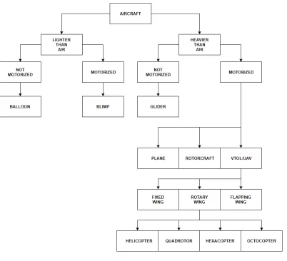
1.4 Quadcopter Classification
There are three subsets of UAVs: fixed wing, rotary wing, and flapping wing, where
quadro-tors are classified under the subset of rotary wing crafts. UAVs are also classified under
motorized aircrafts, under the category ”Heavier Than Air”. [36] [37] A full classification
table is shown in Figure 1.3.
1.5 Brief History of Quadcopters
Earliest attempted designs of a multirotor platform are traced back to Pre-World War II era.
The first recorded multirotor system was a human-operated experimental quadrotor built
by French aircraft designer Louis Charles Breguet, which is reported to have flown a few
times. Another French engineer, Etienne Edmond Oehmichen, developed his own manned
rotorcraft in 1920, which utilized multiple rotor systems to control attitude and forward
thrust. The work done by Oehmichen is credited with leading to the development of tail
rotors, a critical component in modern-day helicopters. In 1922, Dr. George de Bothezat
Figure 1.3: UAV Classification Scheme
their sophistication for their given era, the aforementioned rotorcrafts faced a multitude of
operational and stability issues. Thus, they could not be effectively or practically utilized.
After World War II, some work was done by the US Army to develop manned rotorcrafts.
Some specific examples are theP iasecki V Z−8Airgeep,Chrysler V Z−6, andCurtiss−
W right V Z − 7. Despite preforming well during field testing, the rotorcrafts were not
integrated into service, as they did not meet US Army standards.
In the 21st century, due to the advancement in microelectromechanical systems (MEMS),
micro-controllers, and materials advancement led to a resurgence in multirotor research,
Figure 1.4: Early Multirotor Systems (counterclockwise from top left): Louis Charles Breguet’s aircraft, Oehmichen No.2, de Bothezat helicopter, Curtiss-Wright VZ-7
MEMS and microcontrollers in the present day allows for commercial quadrotors to be built
within a budget, which has enlarged the pool of individuals developing quadrotor platforms
compared to the pool in the 20th century.
Figure 1.5: Modern UAVs
1.6 Multirotor Hardware
A multirotor requires a set of minimal components to achieve flight with additional sensors
and peripherals to supplement requirements of the platform. The core components of a
• Frame/Chassis: A frame serves as the housing for all required components on board
a multirotor. Factors that are taken into account while designing/selecting materials
for a frame are size, weight, strength, and general compatibility with the components
the frame will house. The cost of a frame varies based on the aforementioned factors.
Most modern commercial multirotor frames are built using polymers or carbon fiber
materials. Recent trends have seen frames with power distribution boards integrated
into the chassis (e.g. DJI F450 [38]).
• Rotor system: Multirotor systems require a rotor mechanism to enable flight. The rotor
system is typically comprised of three subcomponents: motors, propellers, and speed
controllers. Modern day multirotor platforms utilize Brushless DC motors (BLDCs),
which require an Electronic Speed Controller (ESC). ESCs are critical components
which ensure proper motor spin rates, which allow for flight. Propellers vary based
on the number of blades, blade pitch, and propeller size, and are chosen based on
the weight of the platform and compatibility with the BLDC. Incorrect choices in
propellers will prevent vehicle flight or may cause suboptimal performance even if
flight is achieved.
• Flight Control System (FCS): The flight control system is responsible for maintaining
stability and ensuring correct operation of all multirotor subsystems. Flight control
units are typically single-board microcontrollers that regulate the rotor speeds based
on sensor feedback. Recently, flight controllers with integrated sensors and ESCs in
a single board have been developed to supplement the increasing demands of micro
UAVs.
• Sensors: The Inertial Measurement Unit (IMU) is the core sensor to any multirotor
platform. A typical 9-DOF IMU is comprised of a 3-D accelerometer, 3-D gyroscope,
of reference. Attitude data obtained through the IMU is used in a feedback loop
into the FCS to stabalize the quadrotor platform. Position sensors, typically Global
Positioning System (GPS) or navigational systems are used to determine quadrotor
platform location. However, position sensors are not a necessity for the operation of a
quadrotor. Other peripherals could include pressure sensors (barometers), motor speed
senors, tilt sensors, etc.
• Power Unit: Typical power supply units for a quadrotor is comprised of nickel or
lithium-based rechargeable batteries, with lithium-based batteries rising to prominence
due to their high energy density and discharge rate. The most commonly used batteries
are lithium-polymer (LiPo) batteries, with other variants including lithium ion
(Li-ion) and lithium iron phosphate (LiFePO4). Modern advancements have also yielded
graphene batteries, which provide longer lifespan, quicker charge time, and higher
capacity, all with less weight than that of the aforementioned batteries.
1.7 Objective
Quadrotors can be used as a versatile robotics platform to test a variety of control
algo-rithms due to their high utility and maneuverability. However, due to a quadrotor’s inherent
instability, a robust control scheme is necessary for effective operation during nominal and
undesired conditions. This thesis proposes a control strategy for a quadrotor under nominal
and fault conditions. The dynamic model is defined through a Newton-Euler formulation and
supporting experimental parameter identification. A dual-loop SMC/PID control scheme is
used for full 6 degrees-of-freedom (DOF) control of the nominal system. In this study,
actu-ator faults on board the quadrotor are interpreted as motor performance losses, specifically
loss in rotor speeds. To control a faulty system, an additive control scheme is implemented in
conjunction with the nominal scheme. The control gains for both nominal and faulty cases
and control based algorithms. The platform developed in this study is used to investigate
the efficacy of quadrotors as Earth-based test platforms for satellite dynamics and control.
1.8 Thesis Overview and Structure
The outline of the thesis is as follows:
• Chapter 2, Dynamic Model of Quadrotor - Overview of the basics of quadrotor
kine-matics and dynamics, experimental validation of parameters, and state space model of
the quadrotor.
• Chapter 3, Quadrotor Control Scheme - Design process of the SMC and PID controllers,
in addition to defining the PSO tuning algorithm.
• Chapter 4, PSO Tuning Process and Results - A walkthrough of the control scheme
gain tuning process with simulation results.
• Chapter 5, Experimental Design of Quadrotor Platform - Design process of the
quadro-tor experimental platform is discussed.
• Chapter 6, Experimental Results - Obtained results from testing the quadrotor
plat-form under a variety of conditions.
• Chapter 7, Proof of Concept Application: Hohmann Transfer - Explores the feasibility
of using quadrotors and other multirotors as Earth-based satellite test platforms.
• Chapter 8, Future Study: Nonlinear State Observer Design for Sensor Fault - An initial
probe into using observer-based techniques for managing sensor faults.
CHAPTER 2
DYNAMIC MODEL OF A QUADROTOR
Figure 2.1: Quadrotor Model
An overall schematic of the quadrotor is shown in Figure 2.1 which introduces the body
and (i.e, Earth) reference frames utilized to derive the translational and rotational dynamics
and kinematics of the quadrotor, based on a Newton-Euler formulation. The body coordinate
frame is defined with thex−y−z orthogonal triad. The Earth coordinate frame is defined
as the North-East-Down (N −E−D) orthogonal triad each representing north, east, and
down, respectively. The red propeller with the rotor speed velocity Ω1 indicates the surge of
the quadrotor platform, while motor with output Ω2 indicates the sway.
intu-itive mathematical model. The assumptions are as follows:
1. The quadrotor frame and affiliated on-board components are rigid.
2. The quadrotor structure is symmetrical.
3. The center of mass of the quadrotor is located at the origin of the body coordinate
axes which lie along the principle axes of inertia.
4. System inputs (generated thrust and drag) are proportional to the square of propeller
velocity.
5. The experimental platform is flying in a closed, laboratory setting.
6. The test bed has slight ground clearance through landing struts, thus ground effects
are considered negligible.
2.1 Coordinate System, Reference Frames, and Rotation Matrices
To define the orientation of the quadrotor body frame with respect to the Earth frame,
Euler’s angles are used. The distance between the body and Earth frame origin is defined
by r = [x y z]. It is assumed that the body and Earth frames coincide and that the order
of rotations follow a 1-2-3 rotation sequence. That is, rotations are about φ (pitch), then θ
(roll), and finally ψ (yaw), a rotation matrix R is derived.
R =
cosθ cosψ sinφ sinθ cosψ cosφ sinθ cosψ+sinφ sinψ
cosθ sinψ sinφ sinθ sinψ+cosθ cosψ cosφ sinθ sinψ−sinφ cosψ
−sinθ sinφ cosθ cosφ cosθ
(2.1)
In practice, it becomes necessary to obtain a relationship between the Euler angle rates
˙
η= [ ˙φθ˙ψ˙] and angular velocity of the body (i.e, body rates) ω= [p q r], shown in Equation
p q r = ˙ φ 0 0 +
1 0 0
0 cosφ sinφ
0 −sinφ cosφ 0 ˙ θ 0 +
1 0 0
0 cosφ sinφ
0 −sinφ cosφ
cosθ 0 −sinθ
0 1 0
sinθ 0 cosθ 0 0 ˙ ψ (2.2)
which reduces to:
p q r =
1 0 −sinθ
0 cosφ sinφ cosθ
0 −sinφ cosφ cosθ ˙ φ ˙ θ ˙ ψ (2.3)
The expression presented in Equation (2.3) can also be written as:
ω=Rrη˙ (2.4)
TheRrmatrix can be reduced to an identity matrix with the assumption that the
quadro-tor predominately operates at hover, or at negligible pitch and roll, therefore small angle
assumption can be made. Thus, the body rates ω are equivalent to the Euler angle rates ˙η.
2.2 System Inputs
On-board brushless DC motors with attached propellers are used to actuate the quadrotor
system. The force Fi and moments Mi generated by the actuators are defined as:
Fi =
1
2ρACTr
2
pΩ
2
i (2.5)
Mi =
1
2ρACDr
2
pΩ
2
i (2.6)
where ρ is the surrounding air density, A is the propeller blade area, CT is the thrust
of motor i = 1, 2, 3, 4.
Equations (2.5) and (2.6) can be simplified to reflect the assumption that generated
system inputs are proportional to the square of the rotor velocity [39].
Fi = KfΩ2i (2.7)
Mi = KmΩ2i (2.8)
where Kf and Km are the aerodynamic force and moment constants, respectively. These
constants are obtained experimentally and are discussed below.
To change attitude states, a torque is applied about the body coordinate axis. This torque
alters the position state and/or the heading of the quadrotor simultaneously, depending on
the nature of change desired from the attitude states. Thus, it is important to note that no
direct inputs control the x and y positions of the quadrotor. To adjust the altitude state,
the total generated thrust by each actuator is summed to determine the overall heave force,
which counters the natural gravitational forces acting on the quadrotor platform.
The total moment acting about each axis of the body coordinate in relation to the rotor
velocities is represented as:
Mx = Kfl(Ω23−Ω 2 1)
My = Kfl(Ω24−Ω 2 2)
Mz = Km(Ω21−Ω 2 2+ Ω
2 3−Ω
2
4) (2.9)
and are categorized as Mb, which represents the overall moments acting on the quadrotor
body frame. The length of the quadrotor arm is represented as l while U2, U3, and U4
Mb = Mx My Mz = lU2 lU3 U4 (2.10)
The applied non-gravitational forces acting on the quadrotor body frame (neglecting
gravitational forces) are defined as:
Fx = 0
Fy = 0
Fz = Kf(Ω21+ Ω 2 2+ Ω
2 3 + Ω
2
4) (2.11)
and are categorized underFb, which represent the overall non-gravitational forces acting on
the quadrotor body frame,
Fb = Fx Fy Fz = 0 0
−U1 (2.12)
where U1 represents the heave force generated by the quadrotor.
The system inputs of the quadrotor are the generated thrust and moments produced by
the rotors on the body-coordinate axes. These inputs are the moments acting about the
x, y, and z axes, along with the non-gravitational force acting on the z axis. Therefore,
the generated force and moments can be related to system inputs through the following
expression, U1 U2 U3 U4 =
Kf Kf Kf Kf
−Kf 0 Kf 0
0 −Kf 0 Kf
Km −Km Km −Km
Ω21
Ω22
where Kf and Km are the aerodynamic force and moment constants respectively.
Thus, the system input vector is defined as:
u= U1 U2 U3 U4 (2.14)
Rewriting Equation 2.13,
u=KAΩ (2.15)
where KA is the aerodynamics matrix and Ω is the squared rotor speed vector.
2.3 Experimental Determination of Aerodynamic Force and Moment Constants
Given the relationship expressed in Equation (2.15), Kf and Km are calculated to generate
accurate system inputs from measured rotor speeds. To accurately determine the
aerody-namic constants, an experimental setup utilizing a load cell and optical tachometer is used to
measure generated forces and rotor speeds, respectively. Given the lightweight nature of the
quadrotor chassis, the required thrust to overcome gravitational and drag forces, along with
rotational forces, are expected to range between 10N-20N (2.25lbf-4.50lbf). These values
are determined based on the range of mass observed across various in-house built quadrotor
platforms. A 25lbf load cell is chosen as the force sensor. A radio transmitter/receiver
sys-tem is used to send throttle signals to the rotor syssys-tems. Throttle is increased incrementally
and the rotor speed and force measurements are logged. Components of Equation (2.13),
specifically U1 and U4, are used to determineKf and Km based on sensor data.
The load cell is calibrated using known masses prior to measurement such that the sensor
sensitivity can be determined. The data points used to determine load cell sensitivity are
N
V and 11.043 N
V , respectively. Averaging the sensitivities term yields the overall sensitivity
value of 11.049 NV . The calibration curves for Kf and Km are shown in Figure 2.2 and 2.3,
respectively.
Testing for Kf requires the quadrotor to generate direct vertical thrust while allowing
for both the load cell and tachometer to measure their respective data. Reflective tape is
adhered to each propeller such that the optical tachometer can measure rotor speed. The
load cell is mounted onto a fixture which allows for the quadrotor platform to rotate about
the vertical axis while allowing for force data to be measured. Figure 2.4 and 2.5 show
placement of the reflective tape and load cell within the experimental setup. Figure 2.6
shows the complete setup for Kf determination. The test platform for Km is such that the
quadrotor is allowed to freely rotate about the z-axis while enabling measurement of the
generated torque. Thus, the load cell is removed from the mount and placed perpendicular
to the quadrotor arm. Figure 2.7 shows the altered setup used to determine Km.
The motor under test is a Turnigy MultiStar 980Kv 14 Pole brushless DC motor.
Mea-sured voltage from the load cell are converted to force values based on the calibration curve
in Figure 2.2. The data acquired from the Kf experimental setup in Figure 2.6 is shown in
in Table A.2 of Appendix A. Based on the U1 component of Equation (2.13), Kf is
deter-mined to be 6.3338×10⁻⁵N-s2. The system input/rotor speed curve used to determineK
f is
shown in Figure 2.8. Similarly, Kf is determined based on the data acquired from the setup
shown in Figure 2.7. For the experimental setup, rotors 1 and 3 were unplugged, such that a
maximum sum of rotor speed could be generated. The system input/rotor speed curve used
to determineKm is shown in Figure 2.9. Utilizing theU4 component of Equation (2.13),Km
Figure 2.2: Load Cell Calibration Curve for Kf Identification
Figure 2.4: Reflective tape applied to quadrotor propeller
Figure 2.6: Kf test experimental setup
Figure 2.8: Rotor Speed/System Input relationship forKf determination
2.4 Rotational Dynamics of Quadrotor
The rotational dynamics is given as:
Mb =J ˙ω+ω×J ω+Mg (2.16)
whereJandMgare the quadrotor diagonal inertia matrix and gyroscopic moments generated
by the actuators, respectively.
The inertia matrix comprises of the moments of inertia about the principle axis on the
body frame of the quadrotor. Ixx, Iyy, and Izz are the principal moments of inertia about
the x, y, and z axes, respectively.
J=
Ixx 0 0
0 Iyy 0
0 0 Izz
(2.17)
The gyroscopic moments are defined as,
Mg =ω× 0 0
JrΩr
(2.18)
where Jr and Ωr are the rotor inertia and relative rotor velocities, respectively. Relative
rotor velocity is defined as:
Ωr =−Ω1+ Ω2 −Ω3+ Ω4 (2.19)
lU2 lU3 U4 =
Ixx 0 0
0 Iyy 0
0 0 Izz
¨ φ ¨ θ ¨ ψ + ˙ φ ˙ θ ˙ ψ ×
Ixx 0 0
0 Iyy 0
0 0 Izz
˙ φ ˙ θ ˙ ψ + ˙ φ ˙ θ ˙ ψ × 0 0
JrΩr
(2.20)
and equating against the angular accelerations, the resulting dynamic model is given as:
¨
φ = l
Ixx
U2+ Jr
Ixx
˙
θΩr+
Iyy
Ixx
˙
ψθ˙− Izz
Ixx
˙
θψ˙ (2.21)
¨
θ = l
Iyy
U3− Jr
Iyy
˙
φΩr+
Izz
Iyy
˙
φψ˙− Ixx
Iyy
˙
ψφ˙ (2.22)
¨
ψ = 1
Izz
U4+Ixx
Izz
˙
θφ˙−Iyy
Izz
˙
φθ˙ (2.23)
2.5 Translational Dynamics of Quadrotor
The translational dynamics of the quadrotor can be expressed as,
m¨r=RFb+mg (2.24)
where m is the mass of the quadrotor system and g is the gravitational acceleration.
Introducing the required terms and expressions to Equation (2.24):
m ¨ x ¨ y ¨ z =
cosθ cosψ sinφ sinθ cosψ cosφ sinθ cosψ+sinφ sinψ
cosθ sinψ sinφ sinθ sinψ+cosθ cosψ cosφ sinθ sinψ−sinφ cosψ
−sinθ sinφ cosθ cosφ cosθ
0 0
and equating against the linear accelerations, the translational dynamics are given as:
¨
x = −U1
m(sinφ sinψ+cosφ cosψ sinθ) (2.26)
¨
y = −U1
m(cosφ sinθ sinψ−cosψ sinφ) (2.27)
¨
z = −U1
mcosφ cosθ+g (2.28)
2.6 Unmodeled Dynamics of the Quadrotor System
As the quadrotor platform is designed to fly in a closed, laboratory setting and have ground
clearance, external disturbances and ground effects are neglected in the modeling process.
Additional physical parameters that influence the dynamics of the quadrotor are turbulence,
vibrations, and air drag. Due to mathematical complexities, limited sensing techniques, and
operating conditions, turbulence from rotor movement/air flow through frame, and vibration
effects are neglected. Therefore, aerodynamic drag becomes the primary contributor of
the unmodeled dynamics for the model in this study, with considerations given to possible
measurement errors made in determination of physical parameters.
Inaccuracies injected into the system through physical parameter imprecision are
classi-fied as structured, or parametric, uncertainties. Such uncertainties in this study result from
errors in calculation of the various inertia terms. Such uncertainties would produce a gain
margin in the control scheme. Accounting for the parametric uncertainties can prove to be a
challenge, as effective measurement of the system to develop reasonable uncertainty bounds
for the parameters is difficult without appropriate equipment. Therefore, to compensate, the
quadrotor model is assembled using Solidworks with added effort to ensure the model is
rep-resentative of the experimental platform. In addition, the gain range for the control scheme
is expanded in order to account for the uncertainties not accounted for in this discussion.
This topic will be discussed in further detail in the upcoming chapter.
as unstructured uncertainties. The lumped uncertainties/unmodeled dynamics of each degree
of freedom is represented asΓi i ∈ φ,θ, ψ,x, y, z and is considered unknown but bounded.
The upper bound ofΓis represented asΓo, such that|Γi| ≤Γo. As the primary contribution
to Γ comes from aerodynamic drag, the upper bound of Γ is equivalent to the maximum drag forceFd experienced by the quadrotor platform.
Usage of the available wind tunnels at the University of New Hampshire in order to
ex-perimentally determine drag parameters were considered. Two wind tunnels were available,
the Student Wind Tunnel and the Flow Physics Facility (FPF). However, due to many
lim-iting factors (including but not limited to scaling issues, quadrotor size, sensor availability,
and site restrictions) made obtaining an experimental aerodynamic profile of the system not
possible. Therefore, a model of the quadrotor platform is constructed through Computer
Aided Design (CAD) software, in which a fluid flow analysis is performed to estimate the
uncertainties of the system. The model used is shown in Figure 2.1.
To perform the fluid flow analysis, SolidWorks Flow Simulation tool is used. The ambient
air settings are modeled at room temperature and at sea level. The maximum drag force
can be determined through a standard drag equation (as in Equation (2.29)).
Fd =
1 2ρv
2C
DAs (2.29)
Given that the quadrotor platform is flown in a closed laboratory setting, the quadrotor’s
speed is limited to 10m/s for safety purposes. First, the maximum drag force felt by the
quadrotor during direct ascent is discussed, where the largest surface area As is exposed
to high fluid velocity. Using Equation (2.29) and parameter values listed in Table 2.1,
the SolidWorks Flow Simulation is initialized to determine the drag coefficient CD and the
maximum drag forceFd felt during direct vertical ascent.
The velocity profile during vertical ascent shown in Figure 2.10, through which CD and
Table 2.1: Drag Upper Bound Calculation Parameters
ρ 1.204 kg/m3
v 10 m/s
As 0.154 m2
Figure 2.10: SolidWorks Flow Simulation Velocity Profile during Vertical Ascent
upper bound as that of the z-axis, since the quadrotor is not capable of moving in lateral
motion without changing attitude. As this exposes a larger surface area to the fluid flow,
the upper bound of Γx and Γy are both set to Γz.
Table 2.2: Calculated CD and Fd Upper Bound for x, y and z through Flow Simulation
Parameter Unit Maximum Value
Fx N 0.007
Fy N -0.033
Fz N 2.514
CD No Unit 0.271
beam, as shown in Figure 2.11. The distributed load is represented as q.
Figure 2.11: Cantilever Beam Representation of Quadrotor Arm
The distributed loadqis approximated as the maximum drag force induced during vertical
ascent in the z-axis applied over the length of the arm, such that:
q= Fz,max
l (2.30)
The maximum moment induced along the quadrotor arm will occur at the fixed point,
while the free end will feel negligible torque. As the rotors are mounted on the free end, they
produce the counter torque required for pitch and roll maneuvers. Therefore, the maximum
moment induced by drag forces which affect the dynamics ofφandθ are determined through
the expression:
MA=
1 2ql
2 (2.31)
where MA is the maximum moment at the fixed cantilevered end.
To determine the maximum moment that can be induced by crosswinds for the yaw
motion, another flow simulation is utilized through SolidWorks Flow Simulation. In this
case, a crosswind flow of 10m/s is induced in the x-axis.
The upper bounds of pitch, roll, and yaw moments are presented in Table 2.3.
Figure 2.12: SolidWorks Flow Simulation Velocity Profile during Crosswind
Table 2.3: Calculated Moment Upper Bound for φ, θ and ψ through Flow Simulation
Parameter Unit Maximum Value
Mφ N-m 0.214
Mθ N-m 0.214
Mψ N-m 8.7×10⁻⁴
Table 2.4: Uncertainty Upper bound
System Uncertainty Units Uncertainty Upper Bound
Γφ N-m 0.214
Γθ N-m 0.214
Γψ N-m 8.7×10⁻⁴
Γx N 2.514
Γy N 2.514
Γz N 2.514
2.7 Unified Dynamic Model
The state vector of the quadrotor is defined as X = [φ φ θ˙ θ ψ˙ ψ x˙ x y˙ y z˙ z˙]T. Recall
The overall dynamics of the system, thus, may be represented as:
˙
X = f(X) +B(X)u(t) +Γ(X,u, t, Fd)
Y = CX (2.32)
where f(x) ∈ R12×1, and B(x) ∈
R12×4 are the nonlinear dynamics and input coefficient
matrix, respectively. The output matrix is an identity matrix C ∈ R12×12, and the system
output vector is Y ∈ R12×1. Note that Γ ∈
R12×1is a function of the system states, input,
time, and drag forces. The system parameters are presented in Table 2.5.
Table 2.5: System Parameters
m 1.13 kg
g 9.81 m/s
l 0.225 m
Ixx 0.016 kg-m2
Iyy 0.016 kg-m2
Izz 0.031 kg-m2
Jr 6×10⁻⁵ kg-m2
Kf 6.33×10⁻⁵ N-s2
CHAPTER 3
QUADROTOR CONTROL SCHEME
Figure 3.1: Quadrotor Control Scheme
The proposed control scheme for the quadrotor experimental platform is discussed in
this chapter. A dual-loop control system, shown in Figure 3.1, is developed for
transla-tion and rotatransla-tional motransla-tion, with an additive compensatransla-tion method actively accounting for
any on-board motor performance losses. The control gains are tuned via Particle Swarm
3.1 Nominal Control Method
3.1.1 Inner Loop Attitude Control Scheme
The chosen control method in this research is a Sliding Mode Controller (SMC), a variable
structure nonlinear control method. The SMC control law consists of two components, a
discontinuous and equivalent control term. The discontinuous term ensures that system
tra-jectory are drawn towards the desired state tratra-jectory, while the equivalent term ensures that
the system trajectory remains on the desired state trajectory upon arrival. SMC provides
advantages of providing stability to nonlinear systems, maintaining stability under
mod-eling imprecision, providing robustness to bounded disturbances, and ensuring finite-time
convergence. However, SMC typically generates chattering due to the discontinuous control
term, in addition to generating high frequency control action which can degrade or damage
on-board hardware and excite higher frequency dynamics.
A sliding surface s and system error e are defined, respectively, as:
e=Xd−X (3.1)
s=ce+e˙ (3.2)
where Xd is the desired state value, and c ∈ R 3×3 is the diagonal equivalent control gain
matrix.
The discontinuous control term is defined such that:
˙
s=−K1(s) (3.3)
where K ∈ R 3×1 is the discontinuous control gain vector and 1(s) represents an odd
switching function, such as a signum or saturation function.
only taking into account known dynamics (i.e., neglecting Γ):
˙
s = ce˙+e¨ ˙
s = c( ˙Xd−X˙) + ¨Xd−X¨
˙
s = c( ˙Xd−X˙) + ¨Xd−f0(X)−B0(X)u(t) (3.4)
where f0(X) ∈ R3×1 is the known nonlinear dynamics of the attitude states only and
B0(X)∈R3×3 is the attitude input coefficients. Note that bothf0(X)andB0(X)are the
subsets of f(X)and B(X). The components of B0(X) are physical constants, therefore it is more appropriate to label the input coefficient matrix for the attitude states as B0. The
components of B0 are:
B0 =
l
Ixx 0 0
0 Iyyl 0
0 0 Izz1
(3.5)
By Equation (3.3) and (3.4), and solving for the control input, the SMC control laws is
determined as:
un =B0−1[K1(s) +ce˙+ ¨Xd−f0(X)] (3.6)
As previously mentioned, a distinct disadvantage of the SMC is the chattering
phenom-ena, which may excite high frequency dynamics. To reduce chattering, 1(s) is chosen to be
a saturation function with a defined boundary layer Φi. Note that si are the components of
sfor states i = φ, θ, ψ.
sat(si Φi ) = si
Φi, if | si
Φi| ≤1
sgn(si), if |Φsii|>1
(3.7)
satura-tion funcsatura-tion, such that:
un =B0−1[Ksat(
s
Φ) +ce˙+X¨d−f
0
(X)] (3.8)
The individual nominal SMC control laws are:
U2 = Ixx
l [kφsat( sφ
Φφ
) +cφe˙φ+ ¨φd+
Jr
Ixx
˙
θΩr−
Iyy−Izz
Ixx
˙
θψ˙] (3.9)
U3 = Iyy
l [kθsat( sθ
Φθ
) +cθe˙θ+ ¨θd−
Jr
Iyy
˙
φΩr−
Izz−Ixx
Iyy
˙
φψ˙] (3.10)
U4 = Izz[kψsat(
sψ
Φψ
) +cψe˙ψ+ ¨ψd−
Ixx−Iyy
Izz
˙
φθ˙] (3.11)
3.1.2 Outer Loop Position Control Scheme
A common Proportional-Integral-Derivative (PID) control scheme is used for position control
for the quadrotor. The individual nominal PID position control laws are:
Ux = Kpxex+Kix
Z t
0
exdt+Kdxe˙x (3.12)
Uy = Kpyey+Kiy
Z t
0
eydt+Kdye˙y (3.13)
U1 = Kpzez +Kiz
Z t
0
ezdt+Kdze˙z (3.14)
where Kp, Ki, andKd are the proportional, integral, and derivative gains, respectively.
Note that Ux and Uy are not direct inputs to the system. Rather, they are virtual inputs
that are used in conjunction with U1 to generate desired pitch and roll values. This occurs
due to the highly coupled nature of the quadrotor states. The desired pitch and roll values
are determined through Equation (3.15) [40] [18]. Note that position states do not influence
φd = tan−1
−Uy
p
Ux2+ (U1+g)2
θd = tan−1
Ux
U1+g
(3.15)
3.2 Fault Tolerant Control for Motor Performance Loss
Motor performance losses are the primary concern for on-board faults, specifically with
SMC potentially creating early onset damage to the motors. Such failures will cause
subopti-mal performance and potential total system catastrophic failure. Motor faults are interpreted
as a loss in rotor speeds. Motor effectiveness loss acts effectively as an additive fault injected
as a control input loss. To mitigate the effects of motor-based faults, an additive fault
com-pensation method is developed. The compensating term is added onto the nominal control
efforts to stabilize and control a quadrotor platform under motor fault. The resulting Fault
Tolerant Control (FTC) augmented law is expressed as:
u =un+uf (3.16)
where un is the nominal control input and uf is the fault compensating term. In this case,
un is the control input provided by the faulty quadrotor without any inherent compensating
term, as in Equations (3.9-3.11) and (3.12-3.14).
The degree of performance loss, or fault magnitude, Fi, on motors i = 1,2,3,4 is
charac-terized as:
Fi =
0, Nominal operation of motor
0< Fi <1, Partial loss of motor effectiveness
1, Total loss of motor effectiveness
The magnitude of fault is determined as,
Fi = 1−
Ωm
Ωd
(3.18)
where Ωm and Ωd are the measured and desired rotor speeds, respectively.
The FTC is formulated based on the relationship between system inputs and rotor
ve-locities, shown in Equation (2.13). Therefore, by multiplying the fault magnitude scalars to
the rotor velocities, Equation (2.13) is augmented into the additive FTC law, as shown in
Equation (3.19).
uf =
U1f
U2f
U3f
U4f
=
Kf Kf Kf Kf
−Kf 0 Kf 0
0 −Kf 0 Kf
Km −Km Km −Km
F1Ω21
F2Ω22
F3Ω23
F4Ω24 (3.19)
3.3 Sliding Mode Control Reachability Condition
To test the stability of the SMC for both the nominal case and operation during a fault, the
following condition, known as the sliding condition, must be satisfied,
1 2
d dts
2
i ≤ −ηi|si|
sis˙i ≤ −ηi|si| (3.20)
where ηi is a strictly positive constant. Equation (3.20) states that the squared distance
to the surface si2 decreases along all system trajectories [41]. In addition, Equation (3.20)
guarantees that the system states will reach the sliding surface in a finite time smaller than
3.3.1 Nominal SMC Stability and Gain Range
A Lyapunov energy functionV is used to explore the attractiveness of the sliding surface
of the nominal SMC. Given a Lyapunov candidate,
V = 1 2s
2
i (3.21)
and taking the derivative of the candidate yields:
˙
V =sis˙i (3.22)
To satisfy the sliding condition in Equation (3.20), the dynamic equations are introduced
to the analysis through ˙s.
˙
V =si(cie˙i+ ( ¨Xdi−X¨i))
s( ¨Xdi−f
0
i(X)−B
0
iunj −Γi+cie˙i)≤ −ηi|si| (3.23)
where unj are the components of control vector un wherej = 2,3,4.
By introducing the control law expressed in Equation (3.6) to Equation (3.23), and
canceling out matching terms yields the following expression:
si(−Γi−kisgn(si))≤ −ηi|si| (3.24)
Given that the system uncertainties remain bounded such that |Γi| ≤ Fn, where Fn
is the upper bound components of the system uncertainties, equivalent to the respective
uncertainty upper bound Fn and the positive constant ηi, such thatki =Fn +ηi,
si(−Γi)−(Fn+ηi)|si| ≤ −ηi|si|
si(−Γi)≤Fn|si| (3.25)
the reachability condition of the SMC is concluded. Applying (3.25) across the attitude
states, the range of stable discontinuous control gains is determined such that:
ki ≥Fn+ηi (3.26)
which ensures that the discontinuous control vector K of components ki meets the
reach-ability condition. For a control law with a saturation function, without loss of generality,
a similar Lyapunov methodology can be applied to determine the solution for K such that
the boundary layer Φi is attractive [41].
The equivalent control gain range dictates the speed of convergence to the sliding surface
upon the state trajectory entering the equivalent control regime. Thus, the equivalent control
range can be set depending on the desired performance by the control designer.
3.3.2 Compensated SMC Stability
For a faulty system, the control input represented in Equation (3.16) replaces the nominal
SMC input in Equation (3.23). In this case, the compensating termuf and its components
ufj are treated as a system input with an unknown disturbance but known bound.
si( ¨Xdi−f
0
i(X)−B
0
iun−Γi+cie˙i) ≤ −ηi|si|
si(−Γi−kfisgn(si)−Bi0ufj) ≤ −ηi|si| (3.27)
Similar to the nominal reachability proof, given that the system uncertainties remain
uncertainties, incorporating Γo and the compensating term upper bound. By stating that
the fault discontinuous control gain range is the sum of fault uncertainty upper bound Ffi
and the positive constant ηi, such thatkfi =Ffi + ηi,
si(−Γi−Bi0ufj)−(Ffi+ηi)|si| ≤ −ηi|si|
si(−Γi−Bi0ufj)≤ Ffi|si| (3.28)
and the range of stable discontinuous gains for a faulty system is such that:
kfi ≥Ffi+ηi (3.29)
which ensures that the discontinuous control vectorKf of componentskfi meets the
reach-ability condition.
The maximum velocity output from the quadrotor’s motor is determined to be 1128.88
rad/s. The maximum fault magnitude assigned is 1, relating to a motor that has experienced
total failure, as shown in Equation (3.17). Thus, the upper bound ofFfi can be determined,
and an effective control gain range is obtained.
The stable gain range for the SMC under nominal and fault conditions are shown in Table
3.1. The control gain range of the PID position controller is determined based on empirical,
iterative tuning through PSO, and will be addressed in the next chapter.
Table 3.1: Sliding Mode Controller Stable Gain Range
SMC Gain Nominal Lower Bound
Nominal Upper Bound
Faulty Lower Bound
Faulty Upper Bound
kφ 0.214 60 36.16 60
kθ 0.214 60 36.16 60
kψ 8.7×10⁻⁴ 60 23.84 60
cx 1 5 1 5
Note that the lower gain bounds determined through Lyapunov represent a conservative
bound. Given practical application, it is unreasonable to believe that the lower bound
accounts for all unmodeled dynamics and parametric uncertainties. Therefore, the upper
gain bounds, as shown in Table 3.1, are chosen with those uncertainties in mind, in an effort
to curtail any dynamics that are not accounted for and unforeseen issues that may arise
during experimental development.
3.4 Controller Tuning through Particle Swarm Optimization Method
In order to tune the control gains of both the SMC and PID controllers, Particle Swarm
Optimization (PSO) is used [42]. Note that the stability of the PID controller is determined
empirically, with repeated tuning of the position controller through the Particle Swarm
Optimization (PSO) method. PSO seeks to minimize a cost function based on a set of given
parameters with assigned weights, which yield a set of optimized variables (i.e., tuned control
gains). Consecutive iterations of the PSO algorithm drive the optimization variable to a set
of gains that result in a minimum cost.
Compared to other optimization techniques, such as Genetic Algorithms (GA) or
Gra-dient Descent, PSO holds several advantages in addition to its simplicity, effectiveness, and
ease of implementation. PSO requires no a priori information regarding the optimization
variables or the search space selected by the user. This ease of restriction allows ease of
scalability and for the optimization of complex systems. PSO is also computationally light
and yields results of large-scale simulation in a timely manner.
The PSO algorithm is expressed as:
∆xi(k+ 1) = W(k)∆xi(k) +P(k)r1(k)[Pb,i−xi(k)] +G(k)r2(k)[Gb−xi(k)]
xi(k+ 1) = xi(k) + ∆xi(k+ 1) (3.30)
Pb,i and Gb represent the respective personal/particle and global best for each xassociated
with minimum cost, where the personal best is obtained from each particle while the global
best is determined based on data of the collective swarm. W(k), P(k), and G(k) are the
user-determined inertial, personal, and global weights, respectively. To encourage particles
to randomize their search prior to convergence at the global best,r1 andr2 act as randomly
generated constants that are bounded such that 0 ≤ rp ≤ 1, where p = 1,2.
3.4.1 PSO Algorithm Initialization
To begin the tuning process, the total number of particles Ip and total time step Kc
must be assigned. Increasing both particle and time step improve the results of the tuning
process and provide a further optimized gain set, with the trade-off of increased computation
time. Weights for the PSO algorithm must also be selected appropriately so as to ensure
that particles are given ample opportunity to explore the search space and refine their own
personal best. Concurrently, the weights should allow the particles to converge to the best
global solution upon meeting the end condition for the algorithm. These weights may either
be assigned as constants or as functions of the time step k.
The chosen inertial, personal and global weights assigned to the PSO function are:
G(k) = e
k−Kc Kc
4 (3.31)
P(k) = 1−G(k) (3.32)
W(k) = e −k Kc
4 (3.33)
The PSO weighting functions are bounded during the tuning process such that G(k) ≥ 0,
P(k), W(k) ≥ 1. P(k) is chosen to be initially larger than G(k) in order to encourage
individual particles to pursue their own personal best. At the point where G(k)≥P(k), the
particles begin to converge towards the best solution within the overall search area. W(k)
![Figure 1.1: UNH TableSat 1C Experimental Test Bed [1]](https://thumb-us.123doks.com/thumbv2/123dok_us/9654808.1493288/22.612.190.418.70.271/figure-unh-tablesat-c-experimental-test-bed.webp)
![Figure 4.1: SMC Tuned Gains for ranges shown in Table 3.1 and weights of Equations (4.1)and (4.2) [Kc= 100, Ipi= 30]](https://thumb-us.123doks.com/thumbv2/123dok_us/9654808.1493288/66.612.125.500.432.643/figure-tuned-gains-ranges-shown-table-weights-equations.webp)
![Figure 4.7: SMC-1 Tuned Gains for ranges shown in Table 3.1 and weights of Equations(4.1) and (4.2) [Kc= 10, Ip= 100]](https://thumb-us.123doks.com/thumbv2/123dok_us/9654808.1493288/70.612.120.500.225.426/figure-tuned-gains-ranges-shown-table-weights-equations.webp)
![Figure 4.8: SMC-2 Tuned Gains for ranges shown in Table 3.1 and weights of Equations(4.1) and (4.2) [Kc= 10, Ip= 100]](https://thumb-us.123doks.com/thumbv2/123dok_us/9654808.1493288/71.612.122.499.78.281/figure-tuned-gains-ranges-shown-table-weights-equations.webp)