Using autoregressive integrated moving average models in the analysis and forecasting of mobile network traffic data

(1)

Using autoregressive integrated moving average

models in the analysis and forecasting of mobile

network traffic data

Francis Kwabena Oduro-Gyimah

1,2

* and Kwame Osei Boateng

1

Department of Computer Engineering, Kwame Nkrumah University of Science and Technology, Kumasi, Ghana. 2

Department of Telecommunications Engineering, Ghana Technology University College, Kumasi, Ghana. Accepted 5 December, 2018

ABSTRACT

Developing prediction models for mobile networks have been increasing in recent years, in response to the ever increasing volumes of customer traffic and also to understand the characteristics of traffic pattern. This study seeks to evaluate the forecasting performance of Autoregressive Integrated Moving Average (ARIMA) models by using an empirical data measured from a live High Speed Downlink Packet Access (HSDPA) telecommunication network operator with coverage in the northern part of Ghana. To determine the best ARIMA model, a number of statistical analysis and tests were carried out. The models with the minimum information criteria values were selected: ARIMA (2,1,3), ARIMA (0,1,2) and ARIMA (1,1,1). Comparing the actual and predicted traffic data show that ARIMA (0,1,2) is the best model.

Keywords: Time series analysis, HSDPA, Autoregressive Integrated Moving Average models, mobile network traffic.

*Corresponding author. E-mail: [email protected].

INTRODUCTION

The increasing demand of bandwidth due to the introduction of packet data services in telephone system networks has been a challenge to telephone operators to upgrade their core networks with high capacity network solutions.

The prediction of network traffic plays an important role in designing, optimization and management of modern telecommunications networks (Yu et al., 2013; Klevecka and Lelis, 2009). With the introduction of High Speed Downlink Packet Access (HSDPA) (Anon, 2004), the available bandwidth has taken yet another leap and today’s users can achieve theoretical upload/download speeds up to 4.2 Mbit/s or 13.1 Mbit/s.

HSDPA is commonly known as 3.5G, as it offers no substantial upgrade to the feature set of Wideband Code Division Multiple Access (WCDMA), but improves on the speed of data transmission to enhance those services (Anon, 2004). WCDMA is a mobile technology that improves upon the capabilities of current GSM networks

that are deployed around the world. It is generally refer as 3G technology, or 3rd generation, and it provides newer services like video calling to the traditional call, and text messaging features that are already standardised. Prior to the introduction of HSDPA, WCDMA networks were only capable of reaching speeds of 384 kbps. Although this might be sufficient for most services, customers always want faster speeds, especially when browsing the internet or downloading files. HSDPA allowed speeds above 384 kbps, the most notable of which is 3.6 Mbps and 7.2 Mbps, which a lot of telecommunications companies often advertise. HSDPA is capable of reaching much higher speeds depending on the type of modulation that is being employed. The theoretical maximum speed of HSDPA is up to 84 Mbps (Anon, 2004).

In general, most time series data are found to exhibit non stationary characteristics and therefore a non-seasonal autoregressive integrated moving average

ISSN: 2354-2144

(2)

(ARIMA) model is widely applied in forecasting this pattern (Namin and Namin, 2018; Ratnayaka et al., 2015).

One basic assumption of ARIMA is the ability to model patterns or combination of patterns which are recursive in time series data, therefore determining and deducing these patterns can help in forecasting (Marek et al., 2008; Haviluddin and Alfred, 2014).

ARIMA models have been described as the most appropriate type for examining these trends because of its ability to adjust to well-balanced statistical assumptions (Ratnayaka et al., 2014; Lee and Tong, 2012). In addition, ARIMA models are described as the most efficient and applicable for experimental data analysis when characteristics of normality, linearity and stationarity postulations are considered (Chen, 1994).

ARIMA models retain high power of predictability with minimal error (Iqbal and Naveed, 2016). ARIMA models are quite flexible in that they can represent several different types of time series and also have the advantages of accurate forecasting over a short period of time and it is easy to implement (Khashei and Bijari, 2011).

A traditional prediction modelling technique that has enjoyed massive usage is ARIMA which is selected for this study owing to the non-stationary characteristics of the collected HSDPA traffic data set (Ratnayaka et al., 2014; Lee and Tong, 2012; Chen, 1994).

Prediction of HSDPA traffic has been growing in recent years. For example, Lawal et al. (2016) applied neural network ensemble to investigate traffic pattern of HSDPA using 690 data points made up of aggregated hourly measurement and concluded that the proposed model predicts well. Abdulkarim and Lawal (2017) also applied the cooperative neural network method to develop forecasting model for HSDPA traffic and user throughput data. Tan et al. (2008) examined the 3G network capacity, the throughput and delay performances of IP-based applications over 3G and HSDPA networks. Khan (2017) experimented with a single site traffic data and countrywide sites traffic data from 3G cellular network in Pakistan and concluded that ARIMA models perform better when the countrywide scenarios are considered while exponential smoothing models give better performance for a single site scenario.

Previous studies on the statistical characteristics of 3G mobile traffic data have identified the presence of self-similarity (Yadav, 2011) and long range dependence (Zhou et al., 2006), therefore suggested that linear models cannot give appropriate prediction. For instance a study by Yu et al. (2013) identified multifractal characteristics in 3G mobile network and applied a combined ARMA and FARIMA model to forecast the traffic. The results indicated that ARMA and FARIMA models are not capable of predicting 3G downlink traffic due to the inherent self-similarity and multifractal characteristics. Svoboda et al. (2008) applied four different methods: linear, exponential regression, and two

Afr J Eng Res 2

more sophisticated ARMA and Dynamic Harmonic Regression (DHR) to forecast packet switched traffic from live 3G networks. The results showed that sophisticated ARMA and DHR models deliver a better performance.

On the contrary this study seeks to evaluate the performance of ARIMA models by using empirical data from a HSDPA network operator which covers the northern sector of Ghana.

RELATEDWORKS

Several researches have been done in the prediction of traffic patterns in 3G networks (Zhang and Cuthberth, 2008). Tso et al. (2010) presented an empirical study on the performance of mobile HSPA networks in Hong Kong. In contrast, Paul et al. (2011) studied traffic dynamics in cellular data networks and focused purely on data traffic in the context of resource usage and subscriber behaviour. The work of Yao et al. (2008) evaluated mobile bandwidth predictability for HSDPA networks using information theory, entropy and concluded that the bandwidth uncertainty reduces drastically when observations from past trips are used to predict bandwidth.

Mäder and Staehle (2006) studied the received interference in HSDPA and proposed a semi-analytical approach to calculate the spatial distribution of the received interference. Their method analysed the interference generated in the own cell and in the surrounding cells including the load dependent interference coming from the dedicated channel users.

In Svoboda et al. (2008), a large-scale cell based measurement analysis of the user behaviour in a live operational HSDPA network was presented. Their research work concentrated on statistical properties of users in cells for refining network planning procedures and to provide realistic traffic models for simulations of cellular packet-oriented networks. Their results suggested four different models which show that conventional simulation settings can lead to an overestimation of performance.

Laner et al. (2012) measured 3G uplink delay in an operational HSPA network and showed that the average delay is strongly dependent on the packet size. They found that last mile delay constitutes a large fraction of measured delays.

In addition, El Bouchti and Haqiq (2011) also studied analytically and numerically the various parameters of performance (loss probability, average delay of packets, average number of packets in the buffer) of control in HSDPA networks.

(3)

TCP-based non real-time flow via extensive HSDPA simulations. Their results demonstrated that the scheme can guarantee the end-to-end quality of service (QoS) of the real-time streaming flow, whilst simultaneously protecting non real-time flow from starvation resulting in improved end-to-end throughput performance.

In Elmokashfi et al. (2012), an active measurement covering 90 voting locations over a period of 6 months were conducted to determine long-term delay using 3 Norwegian 3G networks data connections. They observed that the delay characteristics of the different operators are very different, and that operator-specific network design and configurations are the most important factors for delays. Their study however, concentrated on RTT of 3G traffic data.

METHODOLOGY

This section gives a brief description of the methods applied in developing the model for the HSDPA daily traffic.

ARIMA (p, d, q) model for HSDPA daily traffic

ARIMA model takes historical data and consist of three parts: an autoregressive (AR) process which maintains memory of past events, an integrated (I) process which makes data stationary for easy forecast and a moving average (MA) process for the memory of forecast errors.

Autoregressive model

The autoregressive model of order p with zero mean, denoted as AR(p) is computed in Equation (1) as Yuan et al. (2016):

= + +⋯+ + (1)

where is the time series, , , … , ( ≠0) are model parameters, is white noise with ~ (0, ). The autoregressive operator is given in Equation 2 as Shiumway and Stoffer (2006):

( ) = 1− − B − … − B (2)

where B is the backward operator.

Moving average model

In moving average (MA) modelling, the lagged values are applied as forecast errors to advance the most recent forecast. In such instances, an MA(1) term takes the current forecast error while the MA(2) term relies on

forecast error of the two current periods, similarly it is applied for higher order terms (Iqbal and Naveed, 2016). The moving average model of order q, MA(q) is provided in Equation 3:

= + + +⋯+ (3)

where is the time series, is existing in the moving average lags, , , … , ( ≠0) are model parameters and is white noise with, ~ (0, ).

The non-seasonal moving average operator is given in Equation 4 as Shiumway and Stoffer (2006):

( ) = 1− − B − … − B (4)

where B is the backward operator.

Autoregressive moving average model

The combined non-seasonal autoregressive and moving average models is called autoregressive moving average (ARMA) model. The ARMA model is given as Ratnayaka et al. (2015) in Equation 5:

1 − ∑

= 1 +

∑

(5) Otherwise written as:

= +⋯+ + + +⋯+ (6)

The ARMA (p, q) model can also be written in Equation 7 as Shiumway and Stoffer (2006):

( ) = ( ) (7)

First order difference equation

In developing the model for the HSDPA traffic data, the series must be stationary. This study applied the differencing approach using Equation 8.

(1− ) = − (8)

To confirm that the series is stationarity or otherwise, a unit root test was conducted using Augmented Dickey Fuller (ADF) test (Bhandari et al., 2018), Philip-Perron (PP) test (Phillips and Perron, 1988) and Elliot-Rothenberg-Stock (ERS) test (Elliot et al., 1996), respectively.

Autoregressive integrated moving average

(4)

1− ∑ (1− ) = 1 +∑ (9)

which is also written as (Bhandari et al., 2018):

( )(1− ) = ( ) (10)

where ( ) and ( ) are the and degree polynomials given in Equations 9 and 10, B is the backward shift operator, d is the differencing, is the time series and is the innovation of the original time series, p, d and q be the order of non-seasonal AR, differencing and MA respectively.

The next step in the modelling process is to determine the order of the AR and MA in model specification by applying the autocorrelation function (ACF) and partial autocorrelation function (PACF) approach as shown in Equations 11 and 12.

The estimated ACF is explained as (Shuona and Biqing, 2014):

=∑ ( ̅)( ̅)

∑ ( ̅) (11)

where, ̅=∑

The PACF is given as (Shuona and Biqing, 2014):

, =

= 1

∑ _,

∑ _, = 2,3, … ,

(12)

where, , = , , ,

The next phase is the parameter estimation of the model in Equation 9. In this study the least square estimation approach was adopted and the best models were selected using t-statistics and p-value. The diagnostic checks were done on the selected model for adequacy by analysing the residual plots, and finally forecasting with the model.

ANALYSISANDRESULTS

Data collection

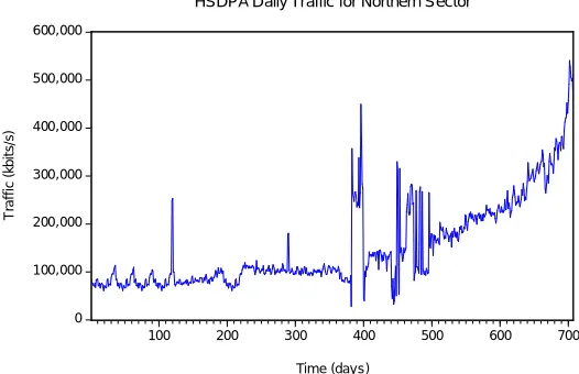
The data for this study is a primary source of daily HSDPA traffic collected from a telecommunications network operator at the Radio network controller (RNC) level covering the northern sector of Ghana. The number of NodeBs that were used in the experiment was 191. The data was collected daily from March 2015 to February 2017. The EViews software and R software were employed for the analysis.

Figure 1 exhibits a non stationarity in the HSDPA daily traffic data. Figure 2 shows the histogram and the statistical description of the HSDPA daily traffic data. The

Afr J Eng Res 4

0 100,000 200,000 300,000 400,000 500,000 600,000

100 200 300 400 500 600 700

HSDPA Daily Traffic for Northern Sector

T

ra

ff

ic

(

k

b

it

s

/s

)

Time (day s)

Figure 1. Time series plot of HSDPA daily traffic data.

0 40 80 120 160 200

100000 200000 300000 400000 500000

Series: Daily_HSDPA Sample 1 707 Observations 707

Mean 152027.7 Median 106289.8 Maximum 540684.2 Minimum 27988.12 Std. Dev. 92867.77 Skewness 1.405012 Kurtosis 4.626256

Jarque-Bera 310.5185 Probability 0.000000

Figure 2. Histogram and statistics of HSDPA daily traffic data.

data is positively skewed with a maximum value of 540684.2 kbps and minimum value of 27988.12 kbps.

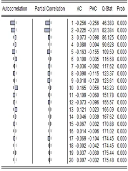
The ACF plot, PACF plot and Q-statistics value of HSDPA traffic for 36 lags are shown in Figure 3. The ACF plot exhibits exponential decay which slowly decreases while PACF plot dies down at lag 3 and no more. From the plot and Q-statistic values, it is clear that the series is not stationary and therefore it must be differenced.

From Table 1, the test statistics of the ADF is less than the critical value therefore the data is not stationary.

(5)

Figure 3. ACF and PACF plot with Q-Statistics values.

Table 1. Test for stationarity of HSDPA daily traffic data using ADF approach.

Test type Constant Trend Constant + Trend

ADF Critical value Test statistic Critical value Test statistic Critical value Test statistic

1% Level -3.440 -0.837 -2.568 0.463 -3.97 -4.502

5% Level -2.866 -1.94 -3.42

10% Level -2.569 -1.616 -3.13

Table 2. Test for stationarity of HSDPA daily traffic data using Philip-Perron approach.

PP Critical value Test statistic Critical value Test statistic Critical value Test statistic

1% Level -3.439 -3.3497 -2.568 0.4917 -3.971 -9.382

5% Level -2.865 -1.941 -3.42

10% Level -2.569 -1.616 -3.13

On the basis of the PP test producing conflicting results, the ERS unit root test was conducted for constant and both constant and trend. From Table 3, ERS test

(6)

Afr J Eng Res 6

Table 3. Test for stationarity of HSDPA daily traffic data using Elliot-Rothenberg-Stock (ERS) approach.

Test type Constant Constant + Trend

ERS Critical value Test statistic Critical value Test statistic

1% Level 1.990 9.0485 3.960 4.093

5% Level 3.260 5.620

10% Level 4.480 6.890

for 5 and 10% level.

Based on the results obtained from the stationarity test, the data was therefore differenced using Equation 8 and the result is shown in Figure 4 which suggests stationarity.

From Table 4, the test statistic of the ADF is greater than the critical values in all three levels; therefore the data can be confirmed to be stationary.

The test results of stationarity using the PP method also confirmed that the traffic data is stationary since the test statistic values are greater than the critical values as illustrated in Table 5.

To further confirm the test, ERS approach was applied to the differenced traffic data, and from Table 6, the data is proven to be stationary.

-300,000 -200,000 -100,000 0 100,000 200,000 300,000 400,000

100 200 300 400 500 600 700

Differenced Daily HSDPA Traffic

T

ra

ff

ic

(

k

b

it

s

/s

)

Time (days)

Figure 4. The first order differenced daily HSDPA traffic data plot.

Table 4. Test for stationarity of differenced HSDPA traffic data using ADF approach.

1% Level -3.4395 -16.4072 -2.568 -16.376 -3.971 -16.446

5% Level -2.8655 -1.941 -3.416

10% Level -2.5689 -1.616 -3.130

Table 5. Test for stationarity of differenced HSDPA traffic data using Philip-Perron approach.

1% Level -3.439 -55.541 -2.568 -54.351 -3.971 -58.244

5% Level -2.865 -1.941 -3.416

10% Level -2.569 -1.616 -3.130

Model identification

From the ACF and the PACF plots of Figure 5, 2 lags are monitored and the rest are not significant. Therefore the following models are selected: ARIMA (2,1,3), ARIMA (0,1,2) and ARIMA (1,1,1).

Parameter estimation

Using the method of least square estimation the

parameters for the selected models are shown in Tables 7, 8 and 9. From the analysis, ARIMA (2, 1, 3) is not statistically significant since the t-value for AR(1) is less than 2, it is therefore rejected. However, ARIMA (0,1,2) and ARIMA (1,1,1) were found to be statistically significant with the absolute t-statistic values greater than 2.

(7)

Figure 5. Differenced ACF and PACF plot of HSDPA.

Table 7. Parameter Estimation for ARIMA (2,1,3).

Variable Coefficient Standard error t-Statistic Prob.

AR(1) -1.190258 0.115929 1.170211 0.0000

AR(2) 0.361436 0.114145 -3.166458 0.0016

MA (1) 0.822970 0.106956 7.694470 0.0000

MA(2) -0.342239 0.085776 -3.989923 0.0001

MA(3) -0.422784 0.050275 -8.409355 0.0000

Table 8. Parameter estimation for ARIMA (0,1,2).

MA (1) -0.384053 0.036693 -10.46656 0.0000

MA (2) -0.237544 0.036723 -6.468474 0.0000

Table 9. Parameter estimation for ARIMA (1,1,1).

AR(1) 0.408321 0.057265 7.130399 0.0000

(8)

Afr J Eng Res 8

Table 10. AIC, AICc and BIC of suggested models.

Model AIC AICc BIC

ARIMA (2,1,3) 10.78833 10.79139 9.82704

ARIMA (0,1,2) 10.78114 10.78404 9.800489

ARIMA (1,1,1) 10.78353 10.78643 9.802879

Diagnostic checking of ARIMA (0.1.2) model

Figure 6 shows the standardised residuals. The standard residuals shows zero mean and few outliers.

The ACF plot in Figure 7 exhibits no proof of significant correlation in the residuals at any positive lag except at 7 and 28. The two lags are however not significant as such the model is adequate.

Forecasting with ARIMA (0,1,2) model

Figure 8 illustrates the plot of the forecasted data and the actual data. The vertical axis represents the HSDPA daily traffic while the horizontal axis represents the time in days. The dashed red lines in the graph represents the actual HSDPA daily traffic while the green line represents the forecast of ARIMA (0,1,2) model. It is clear that the ARIMA (0,1,2) model can predict the HSDPA daily traffic data.

The out-of-sample forecast of traffic data beyond the 700th observation of the ARIMA (0, 1, 2) model is shown in Figure 9. The black line represents the actual data, the red line is the forecast value and the blue line represents the confidence level.

Figure 6. Standardised residual plot of ARIMA (0,1, 2) model.

CONCLUSION

The study has developed ARIMA models to forecast the daily HSDPA network traffic with coverage in the northern sector of Ghana. In achieving these results the models with the minimum information criteria values were selected: ARIMA (2,1,3), ARIMA (0,1,2) and ARIMA (1,1,1). The best model selected out of the three competing models is ARIMA (0,1,2). The model was validated with actual HSDPA daily traffic data and the forecasting results indicated a minor deviation. The

Figure 7. The ACF plot of ARIMA (0,1,2) model residuals.

Figure 8. Graph of actual against forecast data.

Figure 9. Out-of-sample forecast of traffic data.

results agree with an earlier work by Svoboda et al. (2008) and Tan et al. (2008). In addition, the model was

0 200000 400000 600000

1 ₉0

1

79 ₂68 ₃57 ₄46 ₅35 ₆24

T

ra

ff

ic

(

k

b

it

s/

s)

Time in days

Actual

ARIMA (0,1,2)

Time

tr

a

ff

ic

620 640 660 680 700 720

1

0

2

0

3

0

4

0

5

0

6

0

7

0

(9)

used to predict for out-of-sample traffic data. The approach proposed in this study could be helpful to mobile operators in planning and maintaining their HSDPA networks.

REFERENCES

Abdulkarim SA, Lawal IA (2017). A cooperative neural network approach for enhancing data traffic prediction. Turk J Elect Eng Comput Sci, 25: 4746-4756.

Anon. (2004). High Speed Downlink Packet Access; Overall Description. Version 5.7.0, 3GPP TR 25.308.

Bhandari S, Bergmann N, Jurak R, Kusy B (2018). Time series analysis for spatial node selection in environment monitoring sensor networks. Sensors, 18(11): 1-16.

Chen CH (1994). Neural networks for financial market prediction. Proceedings of 1994 IEEE International Conference on Neural Networks (ICNN’94), Orlando, USA, pp. 1199 -1202, 28 June-2 July, 1994.

El Bouchti A, Haqiq A (2011). Access control in multimedia traffic in a 3.5G wireless network. International Conference on Multimedia Computing and Systems (ICMCS), 7-9 April, pp. 1-6.

Elliot G, Rothemberg TJ, Stock JH (1996). Efficient tests for an autoregressive unit root”, Econometrica,64(2): 813-836.

Elmokashfi A, Kvalbein A, Xiang J, Evensen KR (2012). Characterizing delays in Norwegian 3G networks. Simulation Research Laboratory. http://pam2012.ftw.at/papers/PAM2012paper14.pdf.

Haviluddin and Alfred R (2014). Forecasting network activities using ARIMA method. J Adv Comput Networks, 2(3): 173-177.

Iqbal M, Naveed A (2016). Forecasting inflation: Autoregressive Integrated Moving Average Model. European Scientific Journal, 12(1): 83-92.

Khan LU (2017). Performance comparison of prediction techniques for 3G cellular traffic. Int J Comput Sci Network Security, 17(2): 202-205.

Khashei M, Bijari M (2011). Which methodology is better for combining linear and nonlinear models for time series forecasting? J Industrial Syst Eng, 4(4): 265-285.

Klevecka I, Lelis J (2009). Pre-processing of input data of neural networks: The case of forecasting telecommunication network traffic. Teletronika, 3(4): 168-178.

Laner M, Svoboda P, Schwarz S, Rupp M (2012). Users in cells: A data traffic analysis. IEEE Conference on Wireless Communications and Networking, 1-4 April, pp. 3063-3068.

Lawal IA, Abdulkarim SA, Hassan M, Sadiq JM (2016). Improving HSDPA traffic forecasting using ensemble neural networks. 15th IEEE International Conference on Machine Learning and Applications (ICMLA), Anaheim, CA, USA, 18-20 Dec., 2016.

Lee YS, Tong LI (2012). Forecasting nonlinear time series of energy consumption using a hybrid dynamic model. Appl Energy, 94: 251-256.

Mäder A, Staehle D (2006). Interference estimation for the HSDPA service in heterogeneous UMTS networks. Wireless Syst Network Architectures Next Generation Internet, 3883: 145-157.

Marek B, Ondrej K, Emil P, Marek A (2008). A nonlinear mixed effects model for the prediction of natural gas consumption by individual customers.Int J Forecast, 24: 659–678.

Namin SS, Namin A (2018). Forecasting economic and financial time series: ARIMA vrs. LSTM. Machine Learning,pp. 1-19, March.

Paul U, Subramanian A, Buddhikot M, Das S (2011). Understanding traffic dynamic in cellular data networks. In INFOCOM'11, Shanghai, China. www.wings.cs.sunysb.edu/~upaul/paper/Infocom11-final-version.pdf

Phillips PCB, Perron P (1988). Testing for a unit root in time series regression. Biometrika, 75(2): 335-346.

Ratnayaka RMKT, Seneviratna DMKN, Wang Z (2014). An investigation of statistical behaviours of the stock market fluctuations in the Colombo Stock Market: ARMA & PCA approach. J Sci Res Rep, 3(1): 130-138.

Ratnayaka RMKT, Seneviratne DMKN, Jianguo W, Arumawadu HI (2015). A Hybrid Statistical Approach for Stock Market Forecasting Based on Artificial Neural Network and ARIMA Time Series Models. International Conference on Behavioral, Economic, and Socio-Cultural Computing (BESC 2015), pp. 54-60, Nanjing, China, 30 October-1 November, 2015.

Shiumway RH, Stoffer DS (2006). Time series analysis and its applications with R examples. Second Edition, Springer Science+Business Media.

Shuona X, Biqing Z (2014). Network traffic prediction model based on autoregressive moving average. J Networks, 9(3): 653-659.

Svoboda P, Buerger M, Rupp M (2008). Forecasting of traffic load in a live 3G packet switched core network. In: Proc. of 6th International Symposium on CNSDSP, pp. 433–437.

Tan WL, Lam F, Lau WC (2008). An empirical study on the capacity and performance of 3G networks. IEEE Trans Mobile Comput, 7(6): 737-750.

Tso FP, Teng J, Jia W, Xuan D (2010). Mobility: A double-edged sword for HSPA networks. In Proceedings of IEEE (MobiHoc 2010), Chicago, Illinois, USA.

Yadav RK (2011). Modelling of self-similar traffic in wireless networks. In IEEE International Conference on High Performance Computing (HiPC) Proceedings of Workshop on Next Generation Wireless Networks (WoNGeN), Bangalore.

Yao J, Kanhere S, Hassan M (2008). An empirical study of bandwidth predictability in Mobile Computing. In Proceedings of ACM, WiNTECH, pp. 11–18, 2008.

Yerima SY, Al-Begain K (2009). Dynamic buffer management for multimedia services in 3.5G wireless networks. Proceedings of the World Congress on Engineering (WCE 2009), London, U.K, 1 – 3 July.

Yu Y, Song M, Fu Y, Song J (2013). Traffic prediction in 3G mobile networks based on multifractal exploration. Tsinghua Sci Technol, 18(4): 398-405.

Yuan C, Liu S, Fang Z (2016). Comparison of China’s primary energy consumption forecasting by using ARIMA (autoregressive integrated moving average) model and GM(1,1) model. Energy, 100: 384-390.

Zhang K, Cuthberth L (2008). Performing traffic pattern prediction in WCDMA networks. International Conference on Wavelet Analysis and Pattern Recognition (ICWAPR’08), 30-31 August, Hong Kong, China.

Zhou B, He D, Sun Z (2006). Traffic rredictability based on ARIMA/GARCH model. 2nd Conference on Next Generation Internet Design and Engineering (NGI’06), Valencia, Spain, 3-5 April, 2006.

Citation: Oduro-Gyimah FK, Boateng KO (2019). Using autoregressive