^ ST NEUROLOGY
1 9 0 4 1 1 0 3 1 4
A study of the relative-affinity of CSF
antigen-specific IgG in patients with
multiple sclerosis and patients with
encephalitis.
Thesis submitted for the degree of DOCTOR OF PHILOSOPHY
in the
Faculty of Science (Biochemistry), University of London
by
Richard William Luxton
September 1992 Institute of Neurology
ProQuest Number: U063876
All rights reserved
INFORMATION TO ALL USERS
The quality of this reproduction is dependent upon the quality of the copy submitted.
In the unlikely event that the author did not send a complete manuscript and there are missing pages, these will be noted. Also, if material had to be removed,
a note will indicate the deletion.
uest.
ProQuest U063876
Published by ProQuest LLC(2016). Copyright of the Dissertation is held by the Author.
All rights reserved.
This work is protected against unauthorized copying under Title 17, United States Code. Microform Edition © ProQuest LLC.
ProQuest LLC
Abstract
Acknowledgements
I wish to thank my supervisor, Dr. E.J. Thompson for his support and guidance during the practical work and the writing of this thesis, also to Dr. G. Keir for his additional encouragement.
I also thank the staff of the Special Chemical Pathology Department, at the National Hospital for Neurology and Neurosurgery for their help and understanding during this work.
Table of Contents
Abstract ... 2
Acknowledgem ents... 3
Table of Contents ... 4
List of f ig u r e s ... 8
List of ta b le s ... 12
List of p la te s ... 16
List of abbreviations... 17
Section One: Introduction. ... 19
Introduction ... 20
Methods used to study I g G ... 23
Detection of oligoclonal bands ... 23
Quantitative M e th o d s... 26
Methods used to study antigen-specific IgG ... 28
Qualitative T echniques... 28
Quantitative Techniques ... 33
Pathological significance of antigen-specific IgG in the C S F 37 Antibody affinity ... 38
Antigen Binding S ite s... 38
Dispersion F o rces... 44
Hydrogen b o n d s... 44
Hydrophobic b o n d s... 45
Repulsive f o r c e s ... 46
Calculation of affinity c o n s ta n t... 50
Scatchard p l o t ... 52
Langmuir p l o t ... 54
Sips p l o t ... 55
Calculation of Affinity D istributions... 58
Techniques used for measuring a ff in ity ... 61
Equilibrium dialysis ... 61
Ammonium sulphate precipitation... 62
Fluorescent techniques... 62
Solid phase techniques... 64
Measurement of relative affinity ... 67
Dissociative m ethods... 67
Competitive techniques ... 69
Antibody binding methods ... 70
The practical consequences of antibody affinity in solid phase a ss a y s ...71
The biological aspects of antibody a f f in ity ... 73
Antibody affinity and immunopathology... 77
Aim of s t u d y ...79
IgG and albumin measurements... 85
Isoelectric focusing ... 8 6 Isoelectric focusing of antigen-specific I g G ... 87
Development and assessment of new te c h n iq u e s... 89
ELISA screen and method e v alu atio n ... 89
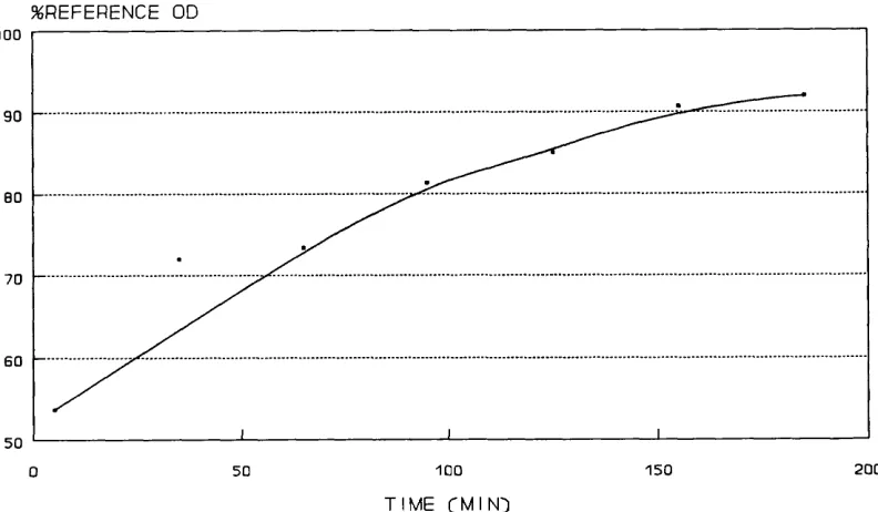
Antigen coating t im e ... 90
The effect of antigen concentration on well coating . . . 92
Sample incubation time ... 96
Detecting a n tib o d y ... 98
Precision studies ... 104
S p ecificity ... 107
Sum m ary... 108
Antigen-specific index ... 109
Measurement of antibody affinity... 113
Quantitation of bound antigen-specific IgG ... 116
Computer M odelling... 122
Measurement of relative affinity ... 124
The effect of sodium thiocyanate on antigen coating . . 129
The effect of sample dilution on affinity distribution . . 131
Blotting methods for antibody affinity ... 133
The effect of w e ig h t... 135
The effect of time ... 135
The effect of antigen d e n s ity ... 136
Section Three: Results from patient sam p les... 140
Introduction ... 141
Initial Study ... 143
Antigen-specific IgG ELISA s c r e e n ... 149
Affinity h isto g ram ... 167
Section Four: Discussion and conclusions. ... 181
Discussion ... 182
ELISA screening t e s t ... 183
Antigen-immunoblots... 187
Antigen-specific Index ... 189
Affinity studies... 193
C onclusions... 199
Future work ... 202
R e fe re n c e s... 203
A ppendices... 229
Appendix A: PASCAL programme for calculating affinity d istrib u tio n ... 230
Appendix B; BASIC programme for calculating the concentration of bound an tib o d y ...235
Appendix C: BASIC programme for calculating relative percentage IgG for the affinity histograms ... 236
Appendix D; Affinity distributions of antigen-specific IgG in patients with multiple sclerosis and patients with viral encephalitis. . . 238
List of figures
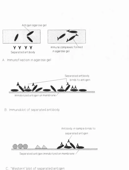
Figure 1.1 Three methods used to study antigen-specific I g G ... 31
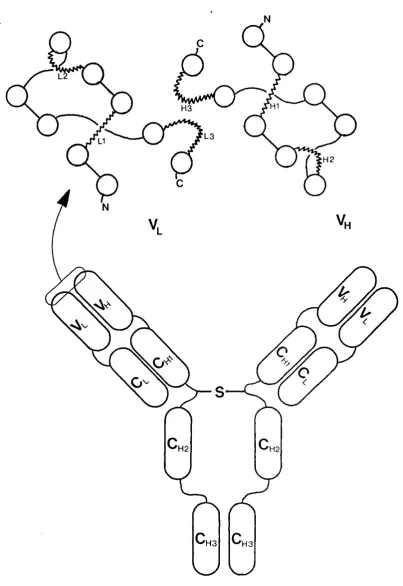
Figure 1.2 Diagram of an IgG molecule showing the antigen binding site with the six hypervariable loops, held in place by strands of B-sheets (open circles). . . . 40
Figure 1.3 Diagram to show the binding site of an antibody that demonstrates high affinity binding (A) and low affinity binding (B)... 47
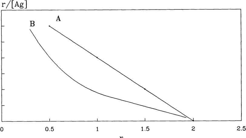
Figure 1.4 Idealized Scatchard plot of hapten bound by monoclonal IgG (A), and polyclonal IgG (B)... 53
Figure 1.5 Langmuir plot showing an ideal linear response... 54
Figure 1.6 Sips plot showing an ideal response... 56
Figure 2.1 Effect of Antigen coating time on optical density... 92
Figure 2.2 Effect of antigen concentration on optical density for measles, herpes and varicella... 94
Figure 2.3 Effect of antigen concentration on optical density after multiple incubations with detector antibody for measles antigen... 95
Figure 2.4 Optical density versus sample incubation time for measles, herpes and varicella... 97
Figure 2.6 Dilution curves for detector antibody for anti-measles IgG in wells coated with measles, measles control antigen and blocking agent... 1 0 1
Figure 2.7 Plot of signal-to-noise ratios against dilution of detector antibody. 102
Figure 2.8 Graph to show the effect of the incubation time of detector antibody, on optical density... 103
Figure 2.9 Plot of signal-to-noise ratio against incubation time of detector antibody... 105
Figure 2.10 Dilution curves of CSF and serum used to calculate antigen-specific index... 1 1 0
Figure 2.11 Diagram showing sandwich technique used in the standard wells to calibrate the amount of antigen-specific IgG remaining in the well after the assay procedure... 115
Figure 2.12 Typical IgG standard curve. IgG concentration in Moles x lO"^®. 117
Figure 2.13 Graph to show computer model of concentration of bound antigen against affinity; with constant antigen concentration of 1 x 10^^® M ... 123
Figure 2.14 Graph to show concentration of bound antibody against total antibody concentration, for different affinities: A =1 x 10^, B=1 x 10®, C = 1 x 10^®,
D = 1 X 10^3... 123
Figure 2.17 Graph to show effect of sodium thiocyanate on the optical density, after 5 and 15 min incubations, without detector antibody... 128
Figure 2.18 The effect of sodium thiocyanate on antigen and blocker (blank) on the well surface... 130
Figure 2.19 Diagram showing structure of coated membrane (A); a band formed from a limited amount of high affinity antibody (B); a band formed from a larger amount of high affinity antibody (C); a band formed from low affinity
antibody (D)... 134
Figure 3.1 Scattergrams of CSF total protein concentration against optical density for: A. Measles, B. Herpes and C. Varicella... 145
Figure 3.2 Scattergrams of CSF IgG concentration against optical density for: A. Measles, B. Herpes, C. Varicella... 146
Figure 3.3 Scattergrams for antigen-specific index calculated from ELISA data and scan data, for MS and encephalitis patients... 165
Figure 3.4a A limited distribution of antibody affinity in CSF and serum from a patient who had a monoclonal IgG pattern by lEF, for anti-varicella IgG. . . 172
Figure 3.4b A limited distribution of antibody affinity in CSF and serum of measles IgG from a patient who had a monoclonal pattern by antigen blot... 173
Figure 3.5 An example of a heterogenous affinity distribution in CSF and serum, this was a case of varicella encephalitis which had a "greater than" pattern by antigen blot... 174
Figure 3.6b Affinity distribution of anti-varicella IgG in CSF and serum from the same patient in figure 3.5a, with HSVE... 176
Figure 3.6c Affinity distribution of anti-measles IgG in CSF and serum from a patient with MS... 177
Figure 3.6d Affinity distribution of anti-herpes IgG in CSF and serum from the same patient with MS as shown in figure 3.6c... 178
Figure 3.7 Scattergrams of patient group against the affinity ratio for CSF and serum... 179
Figure 3.8 Scattergram of patient group against RAV... 180
Figure 4.1 Schematic diagram of the work-flow for antigen-specific IgG
List of tables
Table 1.1 List of some methods used to separate CSF and serum, immobilize and detect antigen-specific IgG, for different antigens in the literature. The letters in brackets refer to the blotting method in figure 1.1... 32
Table 1.2 Attributes of the non-covalent bonds described in the text, (from Laidler and Meiser, 1982)... 41
Table 1.3 The relationship of the association constant and dissociation constant with the equilibrium, or affinity, constant. Data from Steward, 1977... 49
Table 1.4 Comparison of the ranking of affinity values by equilibrium dialysis and ammonium thiocyanate elution. From the study by MacDonald et al (1988). . 69
Table 2.1 Mean blank optical densities for three different detector antibodies . 99
Table 2.2 Within batch precision studies on dilutions of anti-herpes IgG.. . 105
Table 2.3 Precision studies on anti-measles IgG in CSF and serum... 106
Table 2.4 Comparison of precision of coating stage with precision of whole method, n = 9 6 ... 106
Table 2.5 Concentration (mg/1) and the amount of IgG present in the well (moles X 10'^°) for the seven IgG standards... 114
Table 2.7 The relative percentage IgG concentration for each affinity value using three dilutions of CSF, showing change of affinity distribution at each dilution. 132
Table 3.1 Numbers of samples coded into each diagnostic group... 142
Table 3.2 Numbers of patient samples tested by each technique... 142
Table 3.3 The assignment of optical density to a categorical group for the ELISA screen... 143
Table 3.4 Results of Spearman Rank Correlation test for total protein against optical density of the ELISA screen... 144
Table 3.5 Results of Spearman Rank Correlation test for total IgG against optical density of the ELISA screen... 147
Table 3.6 The number of samples which gave a positive reaction against a particular antigen, and the intensity of that reaction... 151
Table 3.7 The number of samples giving a positive reaction against a particular antigen, classified by the total lEF pattern. C + ,S + = identical pattern in CSF and serum, C + ,S -= local synthesis, C+,SO= bands in CSF but no serum results, C + > S + =more bands in CSF than serum, C-,SO= no OCBs in CSF, Para= monoclonal pattern. The numbers in brackets are the number of samples which had both ELISA screen and total IgG blot... 151
Table 3.10 The numbers of samples from each patient group divided into 2 ELISA screen categories according to the strength of reaction. Ctrl= control group. 153
Table 3.11 The number of samples grouped into their antigen-specific IgG and total IgG blot results. L = identical pattern in CSF and serum, 0 = local synthesis, G = more bands in CSF than serum, P = no OCBs in CSF, M = monoclonal pattern... 155
Table 3.12 The number of samples which were trace by ELISA and their antigen blot results... 155
Table 3.13 A-B, Number of samples with a particular blot intensity for MS patients against all antigens (A) (HSVE, SSPE and YE patients were against herpes, measles and varicella respectively), and measles (B)... 158
Table 3.13 C-D, Number of samples with a particular blot intensity, against herpes (C), and varicella (D)... 159
Table 3.14 The number of samples showing local synthesis (LS) by antigen blotting, the encephalitis group was tested against their own antigens, the MS group was tested against all antigens... 160
Table 3.15 The number of patients with and without local synthesis (LS and NO LS) of measles, herpes or varicella IgG by the antigen-specific index (ASI), compared to the number of them which were positive by lEF for total and antigen-specific IgG (ASIgG)... 162
Table 3.17 The range of ASI results found, for measles and herpes specific IgG compared to the ELISA screen intensity... 163
Table 3.18 The number of samples with an ASI less than or equal to 2, and greater than 2, for the different patient groups... 164
Table 3.19 The number of samples which gave the result of local synthesis or leakage by immunoblot (reference method), ASI calculated from scan data and the ASI calculated from ELISA data. An ASI greater than 2.0 was considered to represent local synthesis... 164
Table 3.20 The probability of the null hypothesis being correct for the five equations, for CSF (C) and serum (S) samples from the MS and encephalitis groups. The mean rank for each group is also shown... 170
Table 4.1 Table to show the percentage of MS patients with antigen-specific IgG against the different antigens studied... 185
Table 4.2 The percentage frequency of MS patients with antigen-specific IgG against measles, herpes, rubella and varicella, as reported by other workers, compared to this study... 186
List of plates
List of abbreviations
AGM Arithmetico-geometric mean
ANS 4-anilinonaphthalene- 1-sulphonate
ASI Antigen-specific index
BBB Blood-brain-barrier
BTC Benzethonium chloride
CAACD Chronic antigen-antibody complex disease
CDR Complementary-determining regions
CHIVE Chronic human immunodeficiency-virus encephalitis
CMV Cytomegalovirus
CNS Central nervous system
CSF Cerebrospinal fluid
DANS Dimethylaminonaphthalene-sulphonamide
DNP 2,4 dinitrophenol
ELISA Enzyme Linked ImmunoSorbant Assay
HEEO High electro-endosmosis
HRP Horse radish peroxidase
HSVE Herpes Simplex Virus Encephalitis
IDEA Immunoblot for Densitometric Estimation of Antibodies
lEF Isoelectric focusing
IgD Immunoglobulin-D
IgG Immunoglobulin-G
LIBA Line ImmunoBlot Assay
LS Local Synthesis
ME Medium endosmosis
MS Multiple Sclerosis
PVDF Polyvinylidenedifluoride
RA Relative Affinity
RAV Relative Affinity Value
SLE Systemic lupus erythematosus
SSPE Subacute sclerosing panencephalitis
XT Tetanus toxoid
Section one
Introduction
Cerebrospinal fluid (CSF) is the fluid surrounding the brain, giving it buoyancy and some protection. A human brain weighing 1500 g in air has an effective weight of only 50 g when floating in CSF. The CSF is continually being replaced, bringing some nutrients to the brain and removing waste metabolites. In a normal adult there is approximately 135 ml of CSF being formed at the rate of 350 /xl/min (Cutler et al,
1968), giving an average turnover time of six hours.
The choroid plexuses lying in the third and fourth ventricles (blood-CSF-barrier), produce approximately two thirds of the CSF (Milhorat et al, 1971), the remaining CSF is formed in several extrachoroidal sites (Sato and Bering, 1967) such as the cerebral capillaries (blood-brain-barrier), and dorsal root ganglia. CSF flow is from the ventricles, over the cerebral cortex before being absorbed into the venous blood through the cranial and spinal arachnoid villi. The villi act like a valve only allowing fluid flow in one direction, and thus preventing back flow of blood into the CSF (Welch and Pollay, 1961). The lumber sac containing the spinal cord is a cul-de-sac in which CSF turnover is much slower than ventricular CSF. Using radiolabelled albumin, it has been shown to be 2-4 days (Tourtellotte et al, 1980). For simplicity, in this thesis both barriers are referred as the blood-brain-barrier (BBB).
The normal circulation of lumbar CSF is aided by external compression of the durai sac with respiration and movement; pulsing of parenchyma due to arterial pressure change; and movement of CSF at the ependymal surface by ciliary motion in the ventricles.
protein, the higher the plasma concentration the greater the transfer of protein across the BBB. Secondly, the functional state of the BBB will affect the amount of protein transferred; if there is damage or inflammation of the barrier then there will be increased leakage of protein from the plasma into the CSF (Fishman et al, 1958).
Immunoglobulin-G (IgG) in the CSF is thought to be passively transferred across the BBB, which in a normal individual is approximately 500 times less concentrated than in serum. The concentration of IgG in the CSF can be increased due to higher amounts of plasma IgG getting into the CSF from a primary increase of the plasma IgG concentration, or from damage to the BBB allowing more protein across. Another source of elevated IgG concentrations in the CSF is from local synthesis of IgG within the central nervous system (CNS). Local synthesis of IgG is seen in many different diseases affecting the brain (McLean et al, 1990), including primary demyelinating diseases like multiple sclerosis (MS), and infections of the nervous system (Tourtellotte and Parker, 1966; Link, 1972). To distinguish between local synthesis and leakage of IgG it is necessary to measure the ratio of IgG in CSF and serum, which is then compared with the CSF/serum ratio of a different reference protein. The most commonly used reference protein is albumin (Tourtellotte, 1970; Ganrot and Laurell, 1974; Link and Tibbling, 1977). Other reference proteins have been used, including (X2-macroglobulin (Schliep and Felgenhauer, 1978; Felgenhauer, 1982) and haptoglobin (Baark et al, 1983). If an elevated IgG level in the CSF is due to leakage from the blood, there will be a proportional leakage of reference protein. Therefore dividing the CSF/serum IgG ratio by the ratio for the reference protein corrects for the blood derived IgG and the integrity of the BBB. The CSF/serum IgG ratio divided by the albumin CSF/serum ratio is known as the IgG index (Ganrot and Laurell, 1974).
Examples of these are the Tourtellotte formula (Tourtellotte, 1970); the Schuller formula (Schuller and Sagar, 1981); the Reiber formula (Reiber and Felgenhauer, 1987). The IgG index, and most of the other formulae, need four quantitative measurements, each of which has an analytical and biological variance. This can lead to imprecision of the calculated index.
Methods used to study IgG
IgG methods can be divided into two categories; qualitative techniques that detect the presence of OCBs and quantitative methods that are used in the calculation of the IgG index and other formulae.
Detection of oligoclonal bands
such as jS-trace and 7-trace, can possibly be confused with locally synthesised IgG oligoclonal bands. For a method to be sensitive and specific for IgG an immunostaining technique must be used.
Immunostaining involves the detection of IgG using specific antisera for IgG that is either labelled with an enzyme or radionuclide, alternatively the anti-IgG is detected with a labelled second antibody (Stibler, 1979; Mattson et al, 1980; Kostulas and Link, 1982).
With the arrival of nitrocellulose membranes for immobilizing proteins (Towbin et al, 1979), blotting techniques, with immunostaining, have become widely accepted as the most sensitive method available for detecting OCBs (Walker et al, 1983; Keir et al, 1990). A blotting technique involves transferring the separated proteins from the gel, by either squashing the gel or electrophoresing the proteins from the gel, on to a nitrocellulose membrane. Agarose gels are readily squashed, and collapse under an applied weight, resulting in a near 1 0 0% transfer of protein from the gel on to the membrane (Koch et al, 1985). Polyacrylamide gels, which have a more rigid structure, do not squash easily resulting in an inefficient transfer of protein on to the membrane. Electrophoretic transfer is often used to force the protein from the gel on to the membrane, for which there are several commercial systems available.
It is thought that nitrocellulose binds proteins by hydrophobic interactions. This is supported by the fact that non-ionic detergents such as Triton X-100 or Nonidet P-40 can elute up to 90% of bound protein (Gershoni and Palade, 1982). Ionic interactions are unlikely as the nitro group is uncharged and the binding still occurs in the presence of high salt concentrations. Hydrogen bonding may also contribute to the total binding energy.
Gershoni and Palade (1982) reported a relatively low binding capacity for protein on nitrocellulose (80 /xg/cm^); Millipore technical data reports a protein binding of 251.7 ^g/cm^ for IgG, using their nitrocellulose. Hoffman and Jump (1986) demonstrated that the use of Tween 20 in an immunoblot technique can lead to loss of protein immobilized on the nitrocellulose membrane, as much as 97% being lost in some cases. DenHollander and Befiis (1989) showed that blocking with non-fat milk also led to loss of bound protein, the loss being dependent on the concentration of the milk and the length of time blocking. It was thought that this loss was due to replacement of bound protein with milk protein. To minimize this loss, methods have been described that attempt to fix the protein to the membrane with glutaraldehyde (Jahn et al, 1984; Sharief et al, 1989).
Other membranes have been used for blotting methods such as nylon (Gershoni and Palade, 1982), polyvinylidene difluoride (PVDF) (Nespolo et al, 1987) and epoxy membranes. These have the advantage of being mechanically stronger, and bind proteins with a higher avidity. These membranes can be charge modified, giving a cationic, anionic or hydrophobic membrane and thus they can be selective to which type of molecule will bind. Membranes which bind proteins covalently are now available commercially. These have the great advantage that proteins are not lost during the washing and incubating stages. Manufacturers are reluctant to divulge the nature of the binding reaction; the membranes are a modified PVDF or epoxy membrane. These membranes have the disadvantage of being very expensive relative to nitrocellulose membranes.
anti-IgG. Often enzyme labels are used in the detection system. Horse-radish peroxidase, alkaline phosphatase and glucose oxidase are examples of commonly used enzymes. Other labels used include radiolabels; biotinylated antibodies that form a complex with avidin, giving an increased signal (Kostulas et al, 1987); and luminescent labels that are very sensitive (Laing, 1986).
Quantitative Methods
Local synthesis of IgG in the CNS can be determined from quantitative measurements of IgG in CSF and serum, by applying one of the formulae discussed earlier. The measurement of another protein maybe required. There are many methods that have been used to measure IgG, and other proteins, in CSF and serum, some of which have been automated (Salden et al, 1988). Some methods used in various studies are listed below:
Automated immunoprécipitation and nephelometry;
Kinetic nephelometry;
Electroimmunodiffusion ;
Radial immunodiffusion;
Electrophoresis followed by scanning;
Kostulas et al, 1987 Gallo et al, 1988
Wurster, 1988
Laurell, 1966
Hershey and Trotter, 1980 Caroscio et al, 1983 Keir and Thompson, 1986 Schuller et al, 1987 Luxton et al, 1990
Hische & Van der Helm, 1987
Schuller et al, 1987 Thompson et al, 1983
Thus, if care is not taken, samples with high levels of IgG are recorded as having
lower values. Immunodiffusion techniques; radial immunodiffusion and
Methods used to study antigen-specific IgG
The amount of a particular antigen-specific IgG normally present in blood or CSF is a very small fraction of the total IgG. When a single B-cell is stimulated to divide and produce antibody, as in response to an infection, the antigen-specific IgG synthesised may become a major component of the total IgG. As the concentration of antigen-specific IgG is considerably lower than the concentration of total IgG, more sensitive methods have to be used for its study.
Methods used can de divided into the same categories as the methods used to study total IgG; quantitative and qualitative methods. Qualitative methods involve blotting techniques, usually on to a coated membrane, and give information about the antibody present, that is whether it is polyclonal, oligoclonal or monoclonal. Quantitative methods involve the measurement of concentration or relative concentration, or the titre of antigen-specific IgG. Interest is focused on the presence of locally synthesised IgG within the CNS, therefore antigen-specific IgG is measured in CSF and serum.
Qualitative Techniques
Several techniques have been used that give information about the quality of the
antigen-specific antibody present in the CSF. These methods involved
immune-complexes with the antigen. When polyacrylamide gels were used to separate the CSF or serum proteins, up to five different agarose gels, each containing a different antigen, could be used for antibody transfer. After an overnight wash in saline the agarose gels were pressed under filter paper and rewashed in saline. The press/wash procedure was repeated four times before the gel was incubated with
*^I-anti-human IgG for 12 hours. The plates were washed and dried, the precipitated immune-complexes were visualized by autoradiography for 3 to 24 hours.
Immunoblotting is another widely used technique for the study of antigen-specific IgG. Similar to immunofixation, CSF and serum samples are electrophoretically separated, but then the separated proteins are passed through an antigen coated membrane. Antigen-specific antibody binds to the immobilized antigen, the remaining sample is washed from the membrane leaving the bound antibody ready to be visualized. Some studies have used polyacrylamide gels for the separation step (Karcher et al, 1981; Knisley and Rodkey, 1986; Roos et al, 1987). Other workers have used agarose gel isoelectric focusing followed by immunoblotting which has the great advantage, over polyacrylamide techniques, that there is almost a 100% transfer of sample from the gel to the membrane with no problems of prozoning. The immobilized antigen-specific IgG is visualized using radiolabelled or enzyme labelled anti-human IgG (Moyle et al, 1984; Bukasa et al, 1988; Dôrries et al, 1988; Von Wulffen et al, 1988;).
which particular antigen proteins have antibody raised against them. All the other techniques described show the presence of anti-viral or anti-bacterial IgG, but give no information which viral or bacterial proteins are reacting with the antibody. Another method used to demonstrate the antigen specificity of oligoclonal bands is that of antibody absorption. Here, antigen-specific antibody is removed by the addition of antigen to an aliquot of the sample prior to analysis, by one of the above techniques (Vartdal and Vandvick, 1982; Vandvick et al, 1982). This is then compared with another aliquot which was not adsorbed, looking for differences between the bands. Antigen-specific OCBs would be visible on blot of the non adsorbed sample but absent from the blot of the adsorbed sample.
Antigen agarose gel
Y Y Y Y
Separated antibodyA. Immunofixation in agarose gel
immune complexes formed
in agarose gel
Separated antibody
binds to antigen
Immobilized antigen on membrane
B, Immunoblot o f separated antibody
Antibody in sample binds to
separated antigen
Separated antigen immobilized on membrane
Separation Method AG-EP Blotting Method Detection System AG-IF (A)
Antigen
Measles Rubella Mumps, VZ HSV, CMV Vaccinia Adenovirus Streptococcus
Workers
Vandvik et al, 1979 Vartdal et al, 1980 Vandvik et al, 1982 Vandvik et al, 1985
PG-ffiF NC i^I-Antigen HSV Grimaldi et al, 1988
SDS PG-IEF of antigen
NC(C) Enzyme Campylobacter Von Wulffen et al, 1988
AG-IEF
PG-IEF
coated NC (B) Enzyme
coated NC (B) Enzyme
Measles HIV
Tetanus Diphtheria
Moyle et al, 1984 Dôrries et al, 1988 Bukasa et al, 1988 Knisley and Rodkey, 1986
PG-IEF AG-IF (A) HSV, Munq)s Link et al, 1981 Rubella Rostrôm et al, 1981 Measles Vartdal and Vandvik, 1982 Rotavirus, VZ Sandberg-Wollheim et al, 1987
PG-IEF NC ^^S-antigen TMEV Roos et al, 1987
SDS PG-EP NC (C) Enzyme Sendai virus Kahlon et al, 1987
of antigen HSV Sigmund et al, 1988
SDS PG-EP of antigen
PVDF (C) Enzyme Measles Neumann et al, 1991
A G =agarose E P = electrophoresis PG= polyacrylamide IF = immunofixation
NC= nitrocellulose PVDF= polyvinylidenedifluoride
IE F = isoelectric focusing SDS= sodium dodecyl sulphate
Quantitative Techniques
The detection and quantification of antigen-specific IgG is frequently performed using a solid phase immunoassay technique, where the antigen concerned is coupled to the solid phase. In a solid phase immunoassay antigen is attached non-covalently or covalently to a solid surface (Wood and Gadow, 1983; Hobbs, 1989). Examples of solid phases that have been used in the analysis of antigen-specific IgG are: polystyrene balls (Skoldenberg et al, 1981), polystyrene tubes and cuvettes (Pesce et al, 1977; Leinikki et al 1982), submicron polystyrene particles (Peterson et al, 1989), sepharose (Felgenhaur et al, 1982), polystyrene microplates (Vandvik et al, 1985), polyvinyl microtitre plates (Watt et al, 1988) and nitrocellulose discs (Brankin et al,
1988). Diluted sample, containing antibody, is placed in contact with the solid phase and incubated to allow antibody to bind with the immobilized antigen. After a washing step, when all the unbound antibody is removed from the solid phase, the antigen-specific IgG is detected using a labelled anti-human IgG antibody. Unlike qualitative methods, the intensity of the signal obtained from the captured antigen- specific IgG is measured, giving an indication of the amount of captured antibody on the solid phase.
Quantitative methods have been used for:
• Monitoring levels, and measuring the persistence of antigen-specific IgG, over time, in diseases such as herpes encephalitis (Skoldenberg et al, 1981; Vandvik et al, 1985; Johansson and Blomberg, 1986) and SSPE (Chiodi et al, 1986).
• The comparison of binding activity of antibody to different proteins or peptides (Makela, 1989).
• The comparison of binding activity of antibodies to different antigens in diseases such as multiple sclerosis (Leinikki et al, 1982; Felgenhauer et al, 1985; Hofstad et al, 1987; Persson et al, 1989; Salmi et al, 1989; Dhib-Jalbut et al, 1990).
• A screen for a specific infection, for example TB (Watt et al, 1988), SSPE (Dôrries et al, 1988) and Brucellosis (Araj et al, 1986).
As with total IgG measurement, the ratio of antigen-specific IgG in CSF and serum can be calculated. This in turn can be divided by the total IgG CSF/serum ratio, to correct for leakage of the BBB, as well as differences in IgG concentration in serum versus CSF, which gives the antigen-specific index (ASI).
ASI= — RT
RAS = ratio of antigen-specific IgG in CSF and serum
This approach has the advantage of comparing "like with like," when correcting for BBB function: antigen-specific IgG being compared with total IgG. They are processed identically at the BBB, this is not so for the total IgG index, where total IgG ratio is compared to the ratio of a different protein, for example albumin.
An "idealized" total IgG ratio has been used by Reiber and Lange (1991), which has been produced from an albumin ratio on a theoretical hyperbolic curve, derived from the analysis of normal CSF. This method uses albumin concentrations in the CSF and serum, to produce the "idealized" total IgG ratio, to compare with antigen- specific IgG measurements. As such, this method is not comparing "like with like."
The ASI is a numerical value indicating the amount of local synthesis of antigen- specific IgG. If all the antigen-specific antibody in the CSF is derived from the serum, the ASI will equal 1.0. A value greater than 1.0 would indicate local synthesis of antigen-specific antibody in the CSF. Due to the analytical errors associated with the measurement of the four parameters used to calculate the ASI, different workers have used different threshold values, above which they define the presence of local synthesis of antigen-specific IgG. For example the values of 4.0 (Skoldenberg et al, 1981; Vandvik et al, 1985), 2.0 (Johansson and Blomberg, 1986), 1.5 (Felgenhauer et al, 1988; Neumann et al, 1991) and 1.0 (Mathiesen et al, 1988) have all been used as cut-off values.
In addition to ELISA techniques, there are several methods described that quantify the amount of antigen-specific IgG after separation by an electrophoretic technique. Schadlich et al (1988) described a technique in which antibodies, separated by isoelectric focusing, are quantified by slicing the gel into narrow strips and extracting the antibody. The eluted antibody is measured by ELISA. The areas of anti-measles activity were matched with blots of total IgG. This process was made simpler by the scanning technique called Immunoblot for Densitometric Estimation of Antibodies (IDEA), described by Neumann et al (1991). In this technique antigen was separated by SDS electrophoresis and transferred to a PVDF membrane. Samples of CSF and serum were incubated with a strip of antigen coated membrane and subsequently stained. The intensity of the colour reaction for each band was quantified in a scanning densitometer. The ASI has also been calculated from the areas under densitometric scans of immunoblots of CSF and serum for total IgG and antigen- specific IgG. Appropriate factors were then used to correct for the dilution of serum samples used in the immunoblot technique (Davies, 1988; Paluch et al, 1984).
Pathological significance of antigen-specific IgG in the CSF
Antigen-specific IgG is found in CSF from patients with infections of the CNS, as a result of the immune system responding to the stimulus of a foreign protein. The production of large amounts of antigen-specific IgG is seen as a response to a primary infection in diseases such as herpes simplex virus encephalitis (HSVE) (Vandvik et al, 1982; Grimaldi et al, 1988), subacute sclerosing panencephalitis (SSPE) (Link et al, 1973; Vandvik et al, 1976), varicella-zoster encephalitis (VE) (Mathiesen et al,
1989), chronic human immunodeficiency virus-encephalitis (CHIVE) (Felgenhauer et al, 1988), and mumps meningitis (Salmi et al, 1989). In these conditions, oligoclonal intrathecal synthesis of antigen-specific IgG has been demonstrated, with most of the oligoclonal bands reacting against the antigen causing the primary infection. It has been shown that after HSVE there is a long term persistence of anti-HSV IgG (Vandvik et al, 1985). The presence of antigen-specific antibody directed against antigens other than the primary infective agent has been demonstrated by some workers, who suggest that these other antigen-specific antibodies are due to a "non specific” or "by-stander" immune response during the acute infection (Vandvik et al, 1982; Vandvik et al, 1985; Persson et al, 1989; Salmi et al, 1989).
Antibody affinity
The strength by which an antibody binds to an antigen is described as its affinity for that antigen. Much work has been performed over the past thirty years to understand and measure antibody affinity. An antibody with a high affinity for a particular antigen will bind tightly and be difficult to dissociate from it, whereas a different antibody, with low affinity for that antigen, will bind less firmly and be easier to dissociate.
The terms affinity and avidity are often thought to be equivalent; there is in fact a clear distinction between the two terms. Affinity relates to the strength of binding between a single antibody binding site and its homologous epitope on the antigen. Avidity, on the other hand, relates to the binding strength of the immunoglobulin molecule to the whole antigen, and takes into account antibody and antigen valency, ie. other binding sites, and other secondary factors affecting the binding reaction, for example, interaction between contiguous antibodies which can lead to their mutual stability in the bound state, and therefore are less likely to dissociate.
The terms intrinsic affinity and functional affinity are used by Homick and Karush (1972) to mean affinity and avidity respectively.
Antigen Binding Sites
hypervariable regions which forms the antigen binding site and dictates the specificity and affinity of the antibody (Jones et al, 1986). Recent work suggests that at least five of these hypervariable regions have only a few main-chain conformations, or canonical structures. Changes in the amino acid sequence at a few specific sites would switch the main-chain to another canonical form. Most sequence changes would only modify the surface provided by the side chains on the main-chain of the canonical structure (Chothia et al, 1989). These sequence changes shift the canonical structures, relative to one another, a small but significant amount. Figure 1.2 shows diagrammatically an IgG molecule with the different domains, and an enlargement of the antigen binding site with the hypervariable loops attached to the ends of /3-sheets, represented by the open circles.
Using X-ray crystallography, the shape of the binding site between the L and H chains has been found. Amit et al (1985) have shown the binding site for lysozyme on a hybridoma F(ab) fragment is a concave surface between the H and L chains, which is irregularly undulating. This binding site measures 2 x 3 nm and will take six amino acids or monosaccharide units. On another antibody, the binding site for phosphoryl choline, a small hapten, is in a deep interdomain pocket, probably formed from the /3-sheets (Segal et al, 1974).
H3
L3
H2
H2 H2
H3 H3
Attractive Forces
Electromagnetic interactions between neighbouring molecules give rise to a number of different non-covalent chemical bonds between the molecules. The most important ones involved in antibody-antigen binding reactions are: those involving electrostatic and induced interactions; attractions due to the dispersion effect, for example Van der Waals forces; special electrostatic interaction in the formation of hydrogen bonds; and the interaction between hydrophobic molecules in water. Table 1.2 shows the relative energies in each type of molecular interaction.
Type of bond Typical dissociation
energies KJmol'^
Typical intermolecular distance nm.
ion-ion 680 0.23
ion-dipole 80 0.24
dipole-dipole* 15 0.28
hydrophobic 4 0.30
dispersion 0.25 0.33
* including hydrogen bonds
Electrostatic interactions
Electrostatic, or coulombic, interactions include:
1) Long ranged coulombic interactions between molecules, or groups, with a net charge.
2) Shorter ranged coulombic interactions between noncharged molecules with an
uneven charge distribution, known as dipoles.
3) The interaction between molecules, or groups, which have an induced polarized charge due to fields set up from neighbouring molecules.
One example of an electrostatic interaction, important in protein-protein reactions, is seen between an ionized amino acid and an ionized carboxylic acid.
-NH
3+---
0 0c-The attractive force between two opposite charged ions is proportional to the strength of the charge on the ions, and inversely proportional to the square of the distance separating them.
Where F is the intermolecular force, and Zg are the charges on the two ions and
The attractive force between two dipoles is inversely related to the third power of the distance.
4xr^
Where and are the dipole moments.
In general the interaction energy between multipoles of order n^ and ü2 is described by the formula
Dispersion Forces
These forces arise from molecules without permanent dipole moments, and their origins are described by quantum mechanics. The attractive force arises when two molecules with zero dipole moments are in close proximity. On average the electron cloud is symmetrical, but at any instant a temporary dipole can occur. This temporary dipole will induce a dipole in a neighbouring molecule, at this instant both molecules will have dipoles that will attract each other. The electron clouds surrounding the molecules are in rapid motion and temporary dipoles rapidly fluctuate. There is intermolecular attraction at every instant a dipole is formed, inducing a complementary dipole in a neighbouring molecule. The intermolecular force is proportional to the polarizability (a) and ionization energy of the molecule (E), and inversely proportional to the sixth power of the intermolecular distance.
Dispersion forces in polar molecules are known as Van der Waals forces, and London dispersion forces between non-polar groups. This type of interaction is often the major source of attractive force between many types of molecules.
Hydrogen bonds
30 K J m o l T h e predominant hydrogen bond formed in antibody-antigen binding reactions is that formed between an amino group and a carboxyl group on the different protein strands.
C==0 :
—H-N---If a hydrogen bond is formed between X-H and Y (X and Y are electronegative atoms) then the strength of the bond is proportional to the X-H dipole moment (ji)
and the difference between the ionization potential on atom Y and the noble gas of the same period (A/y), and inversely proportional to the distance between X and Y
at equilibrium (r).
The contribution that hydrogen bonds make towards the total attractive force in antibody-antigen binding is small, especially considering the to competition with water in forming this type of bond.
Hydrophobic bonds
of the hydrophobic bond is an order of magnitude greater than dispersion energy and operates over a range of up to 10 nm. The bonds are important in determining the conformational structure of protein molecules, and are the most important forces in antibody-antigen reactions.
Repulsive forces
In addition to the number of forces described above, which all result in attraction between two molecules, there are repulsive forces at work between molecules.
Repulsive forces operate over a much shorter range than attractive forces and arise when two molecules approach so close, as to cause their electron clouds to interpenetrate and de-shield the nuclei causing separation between the molecules. As the distance separating the molecules decreases the repulsive force % ) increases:
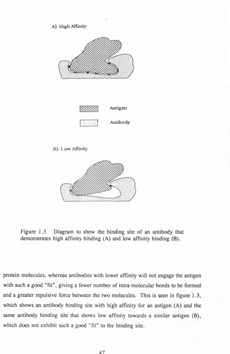
Where B and n are constants and r is the distance separating the molecules. For many molecules the value of n is 12. The shape of the electron clouds of the two molecules is therefore important in determining how close the two molecules can approach before being repelled. This is especially important in the binding of antigen by antibody. If the electron clouds are of a complementary shape at the binding site then the repulsive forces will be kept to a minimum. Conversely where there is a non-complementary 'Tit” the repulsive forces will be high and the attractive forces will be minimized.
A) H igh Affinity
^ Antigen Antibody
B) Low Affinity
Figure 1.3 Diagram to show the binding site of an antibody that demonstrates high affinity binding (A) and low affinity binding (B).
As an antibody molecule binds to an antigen, a number of non-covalent bonds are formed and there is a change in the Gibbs free energy of the system (AG°), at equilibrium Gibbs free energy is at a minimum. The thermodynamic equilibrium constant (K) is related to the change in the standard Gibbs free energy by the equation:
AG° = -RT.lnK
where R is the gas constant and T is the absolute temperature. Here ^ is a dimensionless variable. This relationship expresses the equilibrium constant in thermodynamic terms, measuring changes in energy of the system.
An alternative approach is to calculate the equilibrium constant, by studying the rate reactions of the equilibrium equation. For an antibody-antigen binding reaction this equilibrium can be expressed by the relationship:
A + B ^Z
From these rate reactions a "practical" equilibrium constant can be calculated. In antibody-antigen reactions this equilibrium constant is measured in units of 1/mole.
Association constant M'^ sec'^
Dissociation constant
sec'i
Equilibrium constant M*
1.4 X 10’ 410 1.0 X 10^
1.6 X 10’ 80 1.5 X 10^
8.0 X 10’ 1.4 5.9 X 10^
1.8 X 10* 760 5.8 X 10^
1.3 X 10* 53 2.0 X 10^
1.3 X 10’ 6.4 X 10'^ 3.5 X 10^
1.7 X 10’ 3.4 X 10"* 1.9 X 10*®
Table 1.3 The relationship of the association constant and dissociation constant with the equilibrium, or affinity, constant. Data from Steward (1977).
Calculation of affinity constant
There are several different formulae used in the calculation of the affinity constant for an antibody binding reaction. They are based on the antibody-antigen binding reaction that can be expressed by the equilibrium equation:
Ag+Ab^^AbAg
Where Ag and Ab are the concentration of free antibody and free antigen binding sites respectively; AbAg is the concentration of antibody-antigen complex, is the association constant and is the dissociation constant: this equation does not include antibody or antigen valency, so is a measure of intrinsic affinity of the binding site. At equilibrium the rate of formation of complex is equal to the rate of dissociation; from the law of mass action, which states the rate of formation is proportional to the concentration of reactants, this can be represented thus:
k^[Ab^[Ag]=k^[AbAg^
This can be rearranged to give
^ -K equation 1 K {Ab\\Ag^
The concentration of total antibody (Abj) is the sum of free and bound antibody,
[Abj\ = [Ab] + [AbAg] equation 2
likewise the concentration of the total antigen,
[Ag^^[Ag]-^[AbAg]
These basic equations are combined to produce the Langmuir adsorption isotherm, from which methods for calculating the affinity constant are derived.
Combining equations 1 and 2 and rearrange to obtain:
[AbAg] =K{Abj][Ag]-K\AbAg][Ag]
rearrange and divide by [AbAg] to give:
K[Abj][Ag] \^K [A g
]-[AbAg]
this equation is rearranged to give:
[AbAg] _ K[Ag] [Abj] 1 ^K\Ag]
another form of this equation uses the ratio of bound antibody to free antibody and includes a term for antibody valency in).
Scatchard plot
Scatchard derived his transformation when studying the reaction between small molecules and proteins (Scatchard, 1949). The Scatchard plot is widely used for studying the affinity of antibodies. The equation for the Scatchard plot is derived from the basic equilibrium reaction as follows.
The ratio of bound to free antibody is called r:
[AbAs]
Combine this equation with equation 3 and rearrange to give:
r + rK[Ag]=nK[Ag]
divide by [Ag] and rearrange to give:
= nK -rK
this equation has the form of a straight line.
y=Mx + C
r / [ A g ]
2.5 2
1.5
0.5 1
G
Figure 1.4 Idealized Scatchard plot of hapten bound by monoclonal IgG (A), and polyclonal IgG (B).
When half the total number of binding sites on divalent antibody are occupied, r = l . Then the Scatchard equation becomes:
1
[Ag] = 2K -K
Thus affinity can also be defined as the reciprocal of the antigen concentration when half the number of antibody sites are occupied (r = l ) .
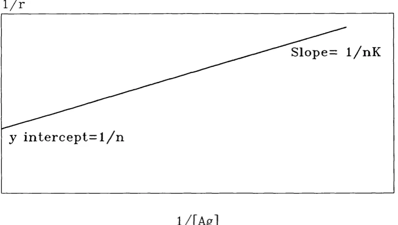
Langmuir plot
The Langmuir equation is derived from equation 5 to give:
1
r K [Ag] n n1 1 L i
Plotting 1/r against l/[Ag] gives a straight line with a slope of 1/nK and a Y intercept of 1/n, see figure 1.5. From this plot the antibody valence and affinity
constant can be obtained.
1 / r
S l o p e = 1 / n K
y i n t e r c e p t = l / n
l / [ A g ]
Also the Langmuir plot can be obtained using the concentration of bound and total antibody:
[AbAg] [Abj] [Ab^
As with the Scatchard plot, this approach to measuring antibody affinity will yield linear results only when using a monoclonal antibody directed against a small hapten. When a heterogenous antibody is used the plot is non-linear. This non- linearity is due to the heterogeneity of affinity constants in the antibody population.
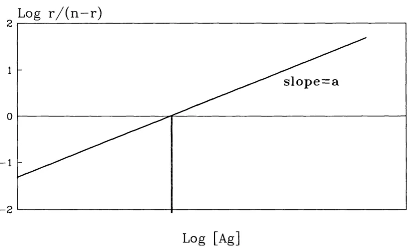
Sips plot
This is a method to quantitate the degree of heterogeneity in an antibody population, which is derived from the logarithmic transformation of the Sips function (Sips,
1948).
n{K[Agl[)-1^(KiAgyf
The logarithmic transformation is:
L o g -J — =aLog[Ag] +aLogK {n-r)
where a is the heterogeneity index and is given by the slope of the line obtained when
Log r/(n-r) is plotted against LogfAg]. Here K is the average affinity constant for the antibody population, which is found when:
An example of a Sips plot is shown in figure 1.6.
A monoclonal population of antibody will give a heterogeneity index of 1. Values less than 1 indicates a heterogenous population, smaller values representing more heterogenous mixtures of affinity constants. This method assumes there to be an unimodal distribution of affinity constants, similar to a Gaussian distribution.
Log r / ( n - r )
s lo p e = a
- 2
Log [Ag]
These methods of measuring antibody affinity assume the antibody and antigen concentrations can be measured accurately and the number of sites on an antibody molecule reacting with the antigen are known; for example, two small hapten molecules react with one molecule of IgG. Much of the investigation into antibody affinity was performed using monoclonal antibodies to hapten molecules like di- nitrophenol.
Calculation of Affinity Distributions
The previous section described how the affinity constant of an antibody can be calculated, but as intimated these methods are best suited to homogenous antibody populations. The Sips equation gives an indication of antibody heterogeneity and an average affinity constant. This average affinity value assumes a normal distribution of affinity values within the given antibody population. There is evidence that suggests that this assumption is invalid. Werblin and Siskind (1972) demonstrated that the affinity distributions of antibody molecules are not generally symmetrical and the data could not be approximated using a Gaussian or Sipsian distribution.
In their study, Werblin and Siskind (1972) used a computer model to calculate the affinity distribution. They divided the antibody population into a number of subpopulations of antibody molecules, each with a different assigned affinity. Using the following equation they calculated the amount of bound antibody (B):
...
where:
equilibrium constant for the subpopulation of antibody. = concentration of antibody sites with affinity constant K^.
C=equilibrium concentration of free hapten or antigen. m=number of antibody subpopulations.
Techniques used for measuring affinity
All the previous methods described for calculating antibody affinity are based on the antibody-antigen equilibrium reaction and the measurement of free, bound or total antibody or antigen, at equilibrium. To measure free and bound antibody or antigen it is essential that they can be distinguished from each other without disturbing the equilibrium of the reaction. This can be achieved by techniques in which the bound and free are physically separate, when measured, or by techniques that use different properties in bound and free enabling one to be measured in the presence of the other. Measurements are made using a range of different antigen concentrations to ensure all the antibody binding sites are saturated. The results can be plotted using one of the techniques previously described.
Equilibrium dialysis
Ammonium sulphate precipitation
In 50% saturated ammonium sulphate solution antibody and antibody-hapten complexes are precipitated (Farr, 1958; Steward and Petty, 1972). Using labelled hapten, bound and free concentrations can be easily derived from the radioactivity measurements in the precipitate and supernatant. This technique is rapid and does not require purified antibody, but can only be used with antigens that are not precipitated with 50% ammonium sulphate.
Fluorescent techniques
Some haptens instead of quenching light emitted from fluorescent amino-acid groups in the antibody, become fluorescent when bound to an antibody. This technique, known as fluorescence enhancement, was first demonstrated by Wrinkler (1962), when he used the hapten 4-anilinonaphthalene-1 -sulphonate (ANS), which is virtually non-fluorescent in aqueous solution but becomes highly fluorescent in hydrophobic solvents. When ANS is bound by antibody in aqueous solution it becomes highly fluorescent, indicating the binding site is a hydrophobic region. Other haptens used are those with a dimethylaminonaphthalene-sulphonamide (DANS) group (Parker et al, 1967), for example DANS-lysine which fluoresces maximally at 520 nm. The intensity of the fluorescence at 520 nm is related to the number of hapten molecules bound. Making measurements with different concentrations of hapten, saturation is reached and ratios of bound and free hapten, at equilibrium, can be calculated. This technique has the advantage over fluorescence quenching methods in that it does not require highly purified reagents because it is an attribute of the hapten that is being measured. The other major advantage of this technique is its usefulness in measuring very low affinity binding reactions because large amounts of hapten can be added to the system, which is non-detectable until it becomes bound to the antibody. Yoo et al (1967) demonstrated that the binding of isolated L chains from rabbit antibody against 4,1-ANS had a binding constant of 1(P 1/mole. L chains from non-specific IgG showed much weaker binding. This technique is only useful for haptens or small antigens that have groups with these particular properties.
the difference between the vertically polarized signal and the horizontally polarized signal, divided by their sum. Values ranged from zero, when the vertical component equalled the horizontal, to one, when the signal was entirely due to the vertical component. Using vertically polarized illumination the emitted intensity was low, so unpolarized illumination was used to excite the sample, thereby giving a more intense signal although the degree of polarization was lower. The greater the polarized signal the more labelled antigen is bound to the antibody. By making a number of measurements at different antigen concentrations, until saturation of antibody is achieved, bound and free ratios can be calculated. This method is useful for haptens and small antigens labelled with a fluorescent label like fluorescein or DANS. Larger antigens have low molecular tumbling rates resulting in a polarized signal, even for free antigen.
Solid phase techniques
Using the equation
anA
a=proportion of available paratopes (antibody binding site). /i=antibody valence.
y4=concentration of total antibody. virus valency.
y = concentration of total virus particles, association constant.
A plot of the left hand side of the equation against anA will give a straight line with a slope of -K^ and an intercept on the x-axis of sV.
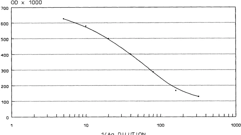
claimed that ELISA methods primarily measured antibody affinity or avidity (Butler et al, 1978). In 1982, using antigen coated microtitre plates, Lehtonen and Eerola found that the use of low sample dilutions, and antibody excess, only those antibodies with higher affinity bound to the antigen. When higher dilutions of sample were used, ie. antigen excess, antibodies with lower affinities would also bind to the immobilized antigen. They also found that antibody with affinity less than 6.3 x 10^ M'^ could not be measured, presumably due to loss during the washing stages. Using this information Lehtonen and Meurman (1982) developed an assay for total and high affinity IgG and IgM against rubella virus.
Beatty et al (1987) measured the affinity of monoclonal anti-CEA with an ELISA technique using serial dilutions of antigen-specific antibody at two different dilutions of antigen, one being half the other. They showed that the total antibody concentration at 100% binding (OD-100) is equivalent to 50% binding (OD-50) when twice as much antigen is used to coat the plate and could use this to calculate the affinity. The affinity constant for the monoclonal antibody was calculated according to the formula
K = ^
2(2[^6']j.-[^6]j.)
[Ab]j is the antibody concentration calculated from the OD-50 and [A b^j is the antibody concentration calculated from the OD-50 for wells coated with half the amount of antigen. This method gives an estimate of the affinity based solely on the concentration of antibody at OD-50 for plates coated with antigen at two concentrations, one half the other. It is quick and practical but only gives good results for monoclonal antibodies.
Several other techniques have been described for measuring antibody affinity in which other methods of separating the bound from the free are used, for example; ultracentrifugation (Normansell, 1970) and gel filtration in sephadex (Stone and Metzger, 1969).
Stanley et al (1983) showed that measurement of antibody is complicated by extreme heterogeneity of the antibody population, and even a very small amount of high affinity antibody in a population of predominantly low affinity antibody will cause an over-estimation of the average affinity and under-estimation of total antibody.
Measurement of relative affinity
There are a number of problems and uncertainties in the measurement of affinity for anti-viral antibodies and many assumptions are made, which may or may-not be correct. Especially when measuring anti-viral, IgG many workers now estimate relative affinity, which involves measuring a quality of the antibody-antigen binding reaction that is affinity dependent and ranking the results on an arbitrary scale. Methods for determining relative affinities can be divided into three groups: dissociative methods, competitive methods and antibody binding methods. Since these methods show relative affinities of subpopulations of antibody within a given population they are more readily adapted to show the distribution of affinities within that population.
Dissociative methods
Antibody dilution curves were constructed in the presence and absence of between 0.5 and 1.0 M guanidine hydrochloride. The resulting optical densities of the two dilution curves were plotted against the dilution, the degree of shift of the dilution curve, in units of log2 was taken to be a measure of affinity. The smaller the shift the greater the overall, or average, affinity. Devey et al (1988) used diethylamine in a similar technique to study anti-tetanus toxoid antibodies.
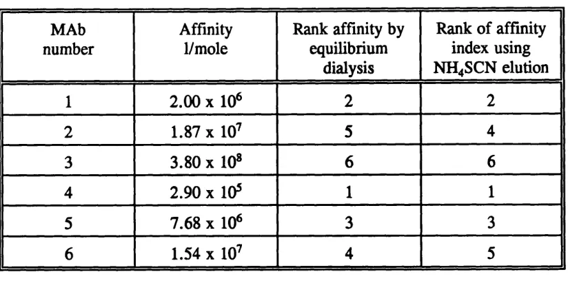
Other techniques used chaotropic agents to dissociate bound antibody from an immobilized antigen. An example being ammonium thiocyanate in the study of avidity of human anti-rubella antibodies (Pullen et al, 1986). In this technique a number of precoated wells, on a microtitre plate, were incubated with fixed dilution of a serum sample. Before detection of bound antibody with a labelled antibody, the wells were washed with increasing strengths of ammonium thiocyanate, 0, 0.5, 1.0, 2.0 and 3.0 mol/1. The optical density in the absence of ammonium thiocyanate was assumed to represent total binding. The optical densities in the presence of the different concentrations of ammonium thiocyanate were expressed as a percentage of total binding. Log^g percentage binding was plotted against the molarity of ammonium thiocyanate. Using a linear regression, the molar concentration of ammonium thiocyanate required to reduce the observed optical density to 50% of the total was taken to be the affinity index. Data was rejected if the optical density of the total binding was less than 0.5 or if the correlation coefficient for the line of best fit was below 0.8 8.
MAb number
Affinity 1/mole
Rank affinity by equilibrium
dialysis
Rank of affinity index using NH4SCN elution
1 2 . 0 0 X 10* 2 2
2 1.87 X 10^ 5 4
3 3.80 X 10» 6 6
4 2.90 X 10* 1 1
5 7.68 X 10* 3 3
6 1.54 X 10^ 4 5
Table 1.4 Comparison of the ranking of affinity values by equilibrium dialysis and ammonium thiocyanate elution. From the study by MacDonald et al (1988).
The elution technique inverted two of the monoclonal antibodies with close affinity values by equilibrium dialysis, otherwise the rankings were equivalent, with a Kendall rank correlation r =0.867, P < 0.02.
Competitive techniques
By plotting the percentage inhibition for each concentration of inhibitor a histogram of the heterogeneity of the antibody was also shown.
Rath et al (1988), using a similar technique studied anti-DNP monoclonal antibodies and compared the affinity value, which was the concentration of free DNP-lysine that reduced the total binding by 50%, to the affinity of the monoclonal measured by equilibrium dialysis. There was a 100% agreement between the ranking of affinity values by the two methods. A histogram of the affinity distribution was plotted as the percentage inhibition achieved by each concentration of free DNP-lysine.
Antibody binding methods
It has been reported that maximum amount of antibody bound to immobilized antigen in a microtitre well can be used for measuring relative affinity (Stone and Nowinski, 1980). Using a fixed concentration of murine leukaemia virus to coat a microtitre plate well, a series of antibody dilutions were set up. Detection of the antibody was with radiolabelled protein A. The maximum amount of antibody that could bind to the coated well was taken as an indicator of the relative affinity of the serum sample. Maximum binding is achieved when all the epitopes on the virus are filled. Any increase in antibody concentration above this point will not increase the observed maximum binding. The fact that different maximum plateaux are observed with different antibodies suggests that this technique is measuring the degree of dissociation that takes place during the washing and detection steps in the assay. Thus the higher the observed maximum binding plateau, the slower the dissociation of antibody. It has been demonstrated that as the coating concentration of virus increases, the sensitivity towards differences in affinity decreases (Nimmo et al,