Moth-Flame Optimization Based Radiant Thermal Pattern Controller For Continuous Stirred Tank Heater

6822

Moth-Flame Optimization Based Radiant Thermal

Pattern Controller For Continuous Stirred Tank

Heater

V. Kabila, G. Glan Devadhas

Abstract: Managing a Continuous Stirred Tank Heater to maintain a uniform temperature within an automated system is complicated. Attaining a constant temperature and sustaining it all through the process is a key challenge inferred in this system. This kind of systems finds its usefulness in many of the automated manufacturing units and in some other chemical processing units too. The controller implemented is meant for regulating the stirring function in order to accomplish a constant actual temperature within the tank. Conventional tuning methodologies trailed to influence the controller experiences various shortcomings in realizing a feasible transient response within the stipulated time. Former Proportional Integral Differential controllers find too hard to organize the entire stirring compartment in a pre-defined manner. Integrating a fuzzy approach augments the delay in proposing a desired value. Those approaches escalated all those necessitated parameters that certainly assists in accomplishing a better performance. In order to overcome all shortcomings inferred, this proposes a Moth Flame Optimization based Radiant Thermal Pattern. Augmented moth-flame optimization methodology tends to initiate the stirring function with a feasible speed and hence, the temperature gets controlled without any delay. The devised approach diminishes the variations of overshoot value in the initial state itself and mitigates the settling time too. The comparative analysis carried out among the suggested mechanism with the traditional approaches like Zeigler-Nicholos, Genetic Algorithm, Particle Swarm Optimization and a hybrid GA-PSO based tuning evidently proves the proficiency in terms of peak overshoot, settling time, rise time and delay time.

Index Terms: CSTH, Moth-Flame, Optimization, Radiant Patterns, Stirred tank Heater, Continuous Stirred Tank Heater, Continuous Stirred Tank Heater

————————————————————

1

INTRODUCTION

Irrepressible need of the hour that typically longs for an automated control system in all sorts of industrial applications serves as a key idea in establishing an optimal controlling system. In order to endow with sufficient power insisted on machinery for a certain amount of time in an unvarying manner, a complete control is acquired through installation of a Proportional Integral Derivative (PID) controller that purposefully serves the industrial ambience without any negotiation. It comprises of prominent and productive features to a vast stretch. One among them is the feedback loops that contributed as a crucial mainstay for alleviating the erroneous inferences incorporated with the processes accomplished in a steady state(Sabir & Ali, 2016).It is literally explored through varied components involved within the deployed PID structure(Jatoth, Jain, & Phanindra, 2013; Rojjananil & Assawinchaichote, 2016)given as proportional gain for unwrapping the errors presently occurred, an integral gain is utilized for unveiling reactive action inferred as a totality of all errors. Finally, derivative gain that is supposed to discover the future samples framed on the basis of the rate assessed with fluctuating errors. This sort of resourceful PID finds its solicitations(Shi, He, Peng, Zhang, & Zhuge, 2016)in several industrious applications such as domestic boilers, solar thermal power generators, biological waste heaters, geothermal power generators, robot manipulators. The real impact of heat energy integrated within these systems are it should get sustained in an unceasing manner right from the beginning until the end of the procedure.

The electrical load assigned to a DC motor is altered into a mechanical energy to provide heat for the devised applications. The applications may infer to accomplish a constant stirring effect or maintain a standard heat or reiterate some sort of without any lag in it. At this juncture, an optimal PID controller is necessitated to manage the overall activities performed by the system in a controlled manner. Intricacies prevalent in all of this conventional PID controller is the accomplishment of tuning constants in accordance with the Proportional ( ), Integral ( ) and Derivative ( )in order to obtain an ideal differential order to sustain the performance. On the occurrence of a high differential order, the computational cost incurred is high. These constants opt for selecting an initial value to fine-tune the metrics through which the controller stability is acquired. If the initial value is precise then the controller stability is accomplished on time without any sorts of additional delay or else the time span incurred for accomplishing controller stability constantly surges up.(Sahib & Ahmed, 2016)discussed several PID parameter tuning methodologies that serve to accomplish an ideal parameter within a precise time span. A conventional methodology trailed to fine tune the PID is given as, Ziegler-Nichols(Shah & Agashe, 2016)stating that the constants are designated on the basis of varied minimizing functionalities and sometimes the overall order of the entire system may get altered. Another PID parameter tuning methodology refers to the Iterative Feedback Tuning (IFT)(Heertjes, Van der Velden, & Oomen, 2016).Though there are many gains acquired owing to its optimized approach, the stability of the entire controlling system is not assured at the time of iterative procedures. The robustness of the whole procedure becomes questionable. Other than these methodologies, some categories of Artificial Intelligence (AI) based procedures are also utilized tune the parameters of PID such as evolutionary algorithm, Differential Evolution (DE) algorithm, Simulated Annealing (SA), multi-objective optimization, Tabu Search (TS), Artificial Bee Colony (ABC) algorithm, fuzzy systems, Particle Swarm Optimization (PSO) algorithm, Many Optimizing Liaisons (MOL) and Genetic Algorithm (GA)(Pi & Ye, 2015; Sharma, Verma, &

_______________________________

• V. Kabila, Research Scholar, Noorul Islam Centre for Higher Education, Kumaracoil, Thucklay. E-mail: [email protected]

6823

Mathew, 2016).The devised objective function incorporates both time as well as frequency metrics to optimize the PID parameters but this results in a minimized overshoot time and a prolonged settling time. The planned Continuous Stirred Tank Heater (CSTH) in employed in a chemical industry that comprises of heat exchangers, pumps, tanks etc. The complete functioning of the deployed tank structure holds the responsibility for accomplishment of the desired chemical reaction at an expected time. The chemical additives utilized usually undergoes varied transitions for every instance of temperature variation. Owing to this property the temperature of the devised tank structure is ought to sustain the temperature at a constant level. Hence in this paper, an optimal controller is opted to manage entire tank structure along with actual temperature maintenance. The paper gets systematized as follows: The comprehensive explanation about the related works on machinery functionality accompanied with the PID controller that is utilized for controlling fluid flow is presented in section II. The implementation process of proposed MFO-RTP based Continuous Stirred Tank Heater (CSTH) is described in section III. The performance of proposed MFO-RTP is scrutinized against the existing algorithms with the various performance parameters in section IV. Latterly, the conclusion in accordance with the proposed methodology for controlling fluid flow in a sustained temperature level is offered in section V.

1.1 Related Works

This section briefly converses the issues in the customized controlling methodologies employed in prior that is implied through manifold controllers to generate the regulated as well as sustained temperature in industrial applications. Lei, et al(Lei, Lin, He, & Zuo, 2013)concentrated on going through Empirical Mode Decomposition (EMD) approach for processing signals in terms of analyzing faults involved machinery rotation on the basis of the time factor. The very basic version of EMD approaches was involved in reiteration of interpolation as well as sifting methodologies that literally incurred a vast time constraint for analyzing the faults in rotors, bearings and gears. Lin and Chen(Lin & Chen, 2013)evaluated an inventive mechanism for investigating the vibration information rehearsed from a rolling bearing that was found operational. Both Mahalanobis Distance Criterion (MDC) as well as Multifractal detrended fluctuation analysis (MF-DFA) were assimilated to design an effectual methodology for unveiling features implanted within time series that were dynamic and non-linear in nature. Crossover functionality was left unconcerned and hence, the conditions deliberated were filed around certain prefixed limits. It was not adaptable with highly fluctuating constraints that were subjected towards varying chemical states of fluids residing in a tank. The features abstracted through the realization of products were not adaptive and compact for analyzing the fault attributes. He, et al.(He, Zi, Chen, Wu, & He, 2015)projected an effective mechanism for examining the faults generated on the rotating bearings of the motors through irrelevant vibrating features designated as Ensemble Super-Wavelet (ESW) transform. Hilbert transform and tunable Q-factor Wavelet Transform (TQWT) methodologies were amalgamated to formulate the ESW in order to unveil the faulty attributes concealed to inhibit the quality of overall performance of the system. The fault signatures and the anomalies inferred with mechanical functionalities were assessed through optimizing parameters

6824

2013). Salazar and Méndez(Salazar & Méndez,

2014)incorporated CO2 for getting operative as a working fluid

in order to examine the transcritical refrigerating cycle through the employment of a lumped energy balance prototype. The preeminent controlling measures were measured by means of utilizing a conventional PID methodology. A viable numerical coding methodology was assimilated to investigate the non-linear system in terms of realizing a robust control measure. However, the evaporator exhibited a feasible control over the operation, the linear methodology devised for managing the overshoots were incapable of deploying control over centrifugal compressors with respect to the supercritical CO2.

The influence of temperature in a recycling procedure is uncontrollable owing to the inference of response delay. Jouppila, et al.(Jouppila, Gadsden, Bone, Ellman, & Habibi, 2014)deployed an operational pneumatic muscle actuator system through an amalgamation of Pulse Width Modulation (PWM) and Sliding Mode Control (SMC) approaches. The deployed methodologies were usually prompted for an enhanced accuracy metric with an incorporation of PWM driven on/off valves in a non-linear systematic model. Li, et al.(Li, Wang, Huang, & Qiu, 2015)utilized a Eulerian model for fabricating a PID controller influenced by an airplane in order to manage the vibration response as well as acoustic nature of the vibro-acoustic cavity implanted within. Two diverse set of techniques were incorporated to manipulate the closed loop control system by means of mitigating the overall dimension of the specific model being framed. Though the noise was immensely controlled, an influence of local optima with respect to varied time-based domain inhibited the anti-interference ability of the controller being designed. Xu, et al.(Xu et al., 2016)recommended a robust Adaptive Fast Fuzzy Fractional Order PID (AFFFOPID) to manage the Pumped Storage Hydro Unit (PSHU) for pursuing the erroneous attributes involved within reversing procedure of energy integrating systems. Bhaskarwar, et al.(Bhaskarwar, Giri, & Jamakar, 2015)concentrated on devising a heat exchanger control structure that was formulated on the basis of tube criterion and shell automation for observing the SCADA platforms through a PID approach. Additional functionality augmented with the PLC-SCADA were data logging facility, set points alterations investigating and exporting the data to a NI-OPC server. LabVIEW prototype was utilized to assess the attributes involved within the entire procedure. Tepljakov, et al.(Tepljakov et al., 2016)evaluated the abruptly altering DC motor control organization along with its dynamics engraved through fractional order dynamic integration. The devised methodology was valid until both the input as well as output signals were retained in a synchronized manner and when the armature winding was incorporated in a series manner with a starter resistor, a significant amount of loss was incurred. Beyond all of the improvements picked up from these established methodologies the limitations inferred were,

 The settling time inferred with devised systems were surging in a constant manner

 Occurrence of instability with the system owing to the tendency exhibited by fluid existing within

 Sustaining the temperature for the whole procedure becomes infeasible relating to the load being augmented or the losses inferred

 Leftover of deliberating the physical functionality system accounts for the faulty inferences.

2

MATERIALS

AND

METHODS

2.1 Proposed MFO-RTP

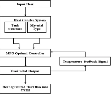
The devised CSTH is realized through the deployment of regular differential equations through which the entire procedure comprising differed inputs at stipulated temperature levels are defined. In general, heat energy is not directly subjected to get into the tank and the jacket layer wrapping it in the outer part i.e., the jacket specified comprises heated fluids that in turn heats the content of the entire tank. Fig. 1 shows the workflow of the proposed MFO-RTP modeling for the regulated temperature.

Fig. 1. Overall flow of MFO-RTP

The expected amount of heat is given into the heat transfer system for processing. The heat passes into the tank is reacted in accordance to the thermal conductivity of the tank material. The heat gained by the tank is due to the stirring function controlled by the deployed MFO optimal controller. The MFO_RTP methodology being employed holds the responsibility for controlling the temperature by mean of getting the temperature from the tank as a feedback signal. Afterward, it performs an optimization in the amount of heat incurred and that optimized form of heat is transferred into the CSTH for accomplishing a constant stirring function.

TABLE 1

TANK MATERIALS USED

Materials Thermal conductivity

Copper 398 w/mk

Aluminium 237 w/mk

Silver 427 w/mk

TABLE 2

DESIGN PARAMETERS OF TANK

Variable Description Value

𝑕 Height 3m

𝑑 Diameter 1.5 m

6825

𝐴 Surface Area 17.6715 m2

𝑣 Volume 5.3014 m3

TABLE 3

DESIGN PARAMETERS OF JACKET

Variable Description Value

𝑕 Height 3 m

𝑡𝑕 Thickness 0.05 m

𝐴 Area 1.5080 m2

Fig. 2. Structure of the CSTH

2.2 Mathematical formulation of the devised CSTH

The heat transmitted to tank from the outward jacket is assessed through manipulation of Heat transmission rate (W) and is given by,

𝑊 = 𝑈. 𝐴 (𝑇− 𝑇), (1)

Where,

Tt and Tjaccount for the temperature in which both tank and

jacket comprise of. The ultimate intention of sustaining the fluid existing within the tank at preferred temperature level is processed through the accomplishment of this tank heater. Straightforward mathematical prototype utilized for completion this CSTH procedure is, material balance as well as energy balance deployed around both jacket and tank. The model of material balance deployed around the tank is given by,

Heat accumulation rate= Input flow rate – Output flow rate ( )

= 𝐹𝑖𝜌 − 𝐹𝜌 (2)

Material balance employed around jacket is specified as, ( )

= 𝐹 𝜌 − 𝐹𝜌 (3)

The model of energy balance employed all over the tank area is indicated as,

Energy mounting up rate = Heat in –Heat out + Heat flow rate

𝑉𝜌𝐶𝑝

= 𝜌𝐹𝐶𝑝𝑇 − 𝜌𝐹𝐶𝑝𝑇 + 𝑊 (4)

Energy balance organized around the jacket is stated as,

𝑉𝜌𝐶𝑝

= 𝜌𝐹𝐶𝑝𝑇 − 𝜌𝐹𝐶𝑝𝑇 − 𝑊 (5)

The devised stirred tank heater is formulated through implication of few constraints defined as,

= (𝑇 − 𝑇) + 𝑈. 𝐴 . ( )

(6)

The control implied for the jacket being surrounded is prompted as,

= (𝑇 − 𝑇) − 𝑈. 𝐴 . ( )

(7)

2.3 Steady State space modelling of MFO-RTP

The conditions implied for accomplishing asteady state criterion is defined as,

𝐹 = 1 𝑓𝑡 3 𝑚𝑖𝑛⁄

2.4 State space modelling of MFO-RTP

Taylor series is utilized to accomplish a state space form by means of transforming the original model into a linear format and it is transfigured as,

= 𝑓1 (𝑇, 𝑇, 𝐹, 𝑇 , 𝑇 ) = (𝑇 − 𝑇) + 𝑈. 𝐴 . ( )

(8)

= 𝑓2 (𝑇, 𝑇, 𝐹, 𝐹, 𝑇 , 𝑇 ) = (𝑇 − 𝑇) − 𝑈. 𝐴 ( )

(9)

On substituting the steady state values in (8) and (9) the differential states of both tank and the surrounding jacket with respect to temperature are defined as,

𝑇̇ = 0 + ,0.4-𝑇𝑡 + ,0.3-𝑇𝑗 + ,−7.5-𝐹𝑡 + ,0-𝐹𝑗 + ,0.1-𝑇𝑡𝑖 +

,0-𝑇𝑗𝑖 (10)

𝑇̇ = 0 + ,3-𝑇𝑡 + ,−4.5-𝑇𝑗 + ,0-𝐹𝑡 + ,50-𝐹𝑗 + ,0-𝑇𝑡𝑖 +

,1.5-𝑇𝑗𝑖 (11)

The state variable are resembled ina standard form stated as,

𝑥̇ = 𝐴𝑥 + 𝐵𝑢 (12)

𝑦 = 𝐶𝑥 + 𝐷𝑢 (13)

The deviated form of input, state and output vectors are specified as,

𝑥 = [_𝑇𝑇 _−𝑇−𝑇

] (14)

𝑢 =

[

𝐹 −𝐹

𝐹 −𝐹

𝑇 −𝑇

𝑇 −𝑇 ]

(15)

𝑦 = [_𝑇𝑇 _−𝑇−𝑇

] (16)

State matrix, 𝑃 = [−0.4 0.3

3 −4.5]

(17)

Input matrix, 𝑄 = [0 −7.5 0.1 0

50 0 0 1.5 ] (18)

Output matrix, 𝑅 = [1 0

0 1] (19)

𝑆 = [0 0 0 0

0 0 0 0] (20)

Type equation here.

Transmuting this defined state space models to the transfer functions in order to sustain the overall temperature of tank in stable manner, differed sorts of parameters are considered such as,

( ) ( )=

. . . . ,

( ) ( )=

. . (21)

( ) ( )=

. . . . ,

( ) ( )=

.

6826

Incorporation of several input parameters for managing the transfer function of jacket wrapping the tank in accordance to temperature of tank by means of controlling the rate of fluid poured in for heating the tank is given as,

( ) ( )=

. . (23)

TABLE 4

DESIGN PARAMETERS INVOLVED IN CSTHPROCESS

Indicating terms Description

V Volume

Cp Capacity of specific heat W Heat transmission rate Ah Area of heat transfer

J Jacket

ref Reference Value

F Rate of change of volume

I Inlet

S Steady value

U Coefficient of heat transfer

Ji Jacket inlet

T Temperature in deg

ρ Density (mass/ volume)

t Time

The algorithm for controlling is listed as follows:

Optimal Controller Algorithm Step 1: Initialize thermal conductivity

𝜍 = 398 𝑤/𝑚𝑘

𝜍 = 237 𝑤/𝑚𝑘

𝜍 = 427 𝑤/𝑚𝑘

Step 2: Define tank details Step 3: Define Jacket details

Step 4: Compute heat transfer coefficient

𝐻 = 𝜍 𝜍 𝑜𝑟 𝜍/𝑡𝑕

Step 5: Compute amount of T increase (o_c)

𝑇 = 𝐻 / 1900 Step 6: Initialize 𝑇 (1) = 0; 𝑇 (1) = 0; 𝑘 = 1 Step 7: for 𝑘 = 1: 𝑇

𝑇 (𝑘 + 1) = 𝑇 (𝑘) + 𝑇 ;

𝑇 (𝑘) = 𝑇 (𝑘 + 1) ;

𝑇 (𝑘) = 𝑇 (𝑘) − 𝑇 ; Construct TF, p= 15/ S2 _{+ 4.9S + 0.9}

Compute Erri = 120 - 𝑇 (𝑘); Erro = 120 - 𝑇 (𝑘) a=1/2;

c1=tf([0 0 a],[1 0]); j=((2*eri)*c1*5)^2; j1=eri+j;

t=(ero*c1)^2; t1=ero+t; d=20;

c2=tf([d 0 0],[1 0]); c3=tf([0 0 d],[1 0]); c4=c2+c3; cj=c4*j1;

T=feedback(cj*p,1); To=feedback(ct*p,1); Tj=Dt*step(T,tm); Tt=Dt*step(To,tm); Temp1(m) = Tj(m); Temp2(m) = Tt(m); k=k+1; end for

The algorithm formulated for optimizing the defined controller works as follows. In the beginning stage itself, the metals being taken for manipulation of a tank is deliberated and is confined with copper, aluminium and silver in accordance its thermal conductivity. Afterward, the tank and jacket details are defined as per the table II and III aforementioned. After then the heat transfer coefficient 𝐻 is computed by trailing the expression,

𝐻 = 𝜍 𝜍 𝑜𝑟 𝜍/𝑡𝑕

Where,𝜍 ,𝜍 and𝜍is thermal conductivity of the tank materials copper, aluminium and silver respectively. At once when the amount of heat being generated is transferred to the tank, the overall temperature intensified within is assessed. Afterward, the amount increase in temperature is computed in each and every instant in both inlet and outlet valves are insisted on by means of initializing and observing the temperature variables as𝑇 and 𝑇 .The temperature optimization procedure is carried out until both temperatures prevailing within inlet as well as outlet valves of the jacket gets regulated. This process gets subjected to the transfer function employed within the CSTH. The temperature being applied is assessed for the error values accomplished from the inlets of both jackets (Erri)

as well as the outlet of tank (Erro). This error value acquired is

analyzed and given as a feedback for controlling system. Now, the control system completely examines the error values in accordance with the tank outlet value and adjusts the temperature given into the inlet valve of a jacket.

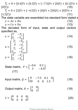
2.5 Controller design description

The controller design for the proposed work is illustrated in Fig.3. The output given as a requisite for the CSTH is fed as the input for the error𝑒(𝑡)and it is further passed into the proposed MFO-RTP controller. During integration procedure, the input given input is minimized if it gets increased beyond the stipulated limit. Likewise, the differentiating portion certainly increases the diminished value during the process of attaining the actual temperature. Afterward, the implemented MFO algorithm is iterated in search of a feasible value to reach the actual temperature.

Fig. 3. Controller design diagram

Implemented MFO-RTP controller achieves an actual temperature at the initial stage itself without any sorts of negotiation in the values. The output values obtained from the transfer function as if specified in (24) is again fed as the input for the error function and a constant stirring function is obtained.

𝑢(𝑡) = ,∫ 𝑒(𝑡) . 𝑑𝑡 ∗ ∫ 𝑒(𝑡) . 𝑑𝑡- + ,𝑑 ( )

- (24)

In this experiment, concerning all the major heat transfer forms there are numerous portions in overall equation. The following equation represents the container heat in and out of

dQ/ dt = U*A*(T1-T) (25)

6827

transfer area, T1 denotes ice bath temperature and T represents inside temperature of the water at any point in time. After this the ideal convection is assumed within the container, the heat quantity of the fluid changes for every interval is labelled as

dQ/dt = 𝜌 ∗𝐶 𝑝 ∗𝑉 ∗𝑑 𝑇 /𝑑 𝑡 (26)

The equation 25 and 26 are combined together and created the below equation

𝑈 ∗𝐴 ∗(𝑇 1−𝑇 )=𝜌 ∗𝐶 𝑝 ∗𝑉 ∗𝑑 𝑇 /𝑑 𝑡 (27)

The variables are separated and integrating it and the temperature affords overall heat transfer equation given below

𝑇 1−𝑇 /𝑇 1−𝑇 𝑖 = 𝑒 ∗ ∗ / ∗ ∗ ₍₂₈₎

The values utilized for variables are The flask dimensions are

(100mL): O.D. by Height: 65 mm by 120 mm; Radius: 0.0325 m

(250 mL): O.D. by Height: 82 mm by 134 mm; Radius: 0.0410 m

(500 mL): O.D. by Height: 103 mm by 174 mm; Radius: 0.0515 m

(1000 mL): O.D. by Height: O.D. by Height: 132 mm by 213 mm;

Radius: 0.066 m

𝐴 =Surface Area (half-sphere): 𝐴 =2𝜋 𝑟 2

𝑉 =Volume (half-sphere) = =23𝜋 𝑟 3

At 10 C, specific heat values and density is involved once it’s about the half-way point among the lowest and highest values of temperature utilized

Cp = 4185.5 J/ kg* K, 𝜌 =999.8𝑘 𝑔 /𝑚 3, 𝑇 1= Ice temperature; 0 °C

13

𝑡 = time taken from 𝑇 𝑖 to 𝑇 in seconds to cool the water

𝑇 = Final temperature of the water while the timer was stopped U = Overall heat transfer coefficient in 𝑊 /𝑚 2∗

𝑇 𝑖 = the highest temperature remains initial temperature of water attained once mixing identical amounts of cold and hot water

The graphical representation of this concept can be plotted as time versus the natural log of 𝑇 1−𝑇 /𝑇 1−𝑇 𝑖 . The slope of graph’s straight position is equal to −𝑈 ∗𝐴 ∗𝑡 𝜌 ∗𝐶 𝑝 ∗𝑉 , in which the surface area and volume of each flask is used for calculating U.

2.6 MFO Algorithm

Incorporation of Moth-Flame Optimization algorithm significantly enhances the entire performance of the employed PID controller towards the attainment of an actual temperature level. It is worked out in a hyper-dimensional space, where the moths tend to alter their position in search of a flame or flag i.e., a feasible solution through its usual movement trailing a transverse orientation. In this scenario, moths usually represent the search agents that move around in search of flags or pins dropped by moths particularly known as flames within a search space. All moths (m) are resembled in a matrix

form owing to its population-based nature.

𝑚 = [

𝑚 _, 𝑚 _, 𝑚 , 𝑚 , ⋯

𝑚 _, 𝑚 ,

⋮ ⋱ ⋮

𝑚 , 𝑚 , ⋯ 𝑚 _,

] (25)

Where d indicates single dimension in which the moths gets traversed and l refers to the number of moths.

The flags are also deliberated in the same format as the moth matrix given as,

𝑓 =

[

𝑓 , 𝑓 ,

𝑓 , 𝑓 ,

⋯ 𝑓 , 𝑓 ,

⋮ ⋱ ⋮

𝑓 , 𝑓 , ⋯ 𝑓 , ]

(26)

Where l specifies the total number of moths and d states the total number of dimensions in which the flags are available. Fitness value for both moths and flags are deposited in respective arrays given by,

𝑂 = [ 𝑚 𝑚 ⋮ 𝑚

]and 𝑓𝐴 = [ 𝑓 𝑓 ⋮ 𝑓

] (27)

Where O designates the fitness function of moths and fA represents the fitness function of flags respectively.

A global optimal of the optimization in the MFO algorithm is provided in a three-tuple function given as,

𝑀𝐹𝑂 = (𝑖, 𝑝, 𝑦) (28)

An arbitrary population of moths as well as the fitness value are created by the function i and is given by,

𝐼: 𝜑 → *𝑚, 𝑂+ (27)

The moths are driven to move around the search space through function p that particularly collects the moth matrix and an updated matrix is returned.

𝑝: 𝑚 → 𝑚 (28)

On reaching a termination condition, the entire search procedure gets terminated and it’s denoted by the variable y.

𝑦 → 𝑚 *𝑡𝑟𝑢𝑒, 𝑓𝑎𝑙𝑠𝑒+ (29)

An arbitrary distribution of values are utilized to create an initial set of solutions on the basis of objective functions. If the moths tend to move out of a defined search space, then it is driven back into a specific search space by,

𝐹𝑙𝑎𝑔 = Moth > 𝑈𝑏 (30)

𝐹𝑙𝑎𝑔 = Moth < 𝐿𝑏 (31)

The fitness function values are formulated on the basis of those objective function given as,

𝑚 _, = (𝑢𝑏(𝑔) − 𝑙𝑏(𝑔)) ∗ 𝑟𝑎𝑛𝑑() + 𝑙𝑏(𝑔) (30)

At once when those distributions are initiated, 𝑝 is reiterated until the satisfying criterion 𝑦 is met. Location of each and every moth is regularly updated in accordance with the position held by each flag and that updating procedure is given as,

Moth = Moth ∗ (~(𝐹𝑙𝑎𝑔 + 𝐹𝑙𝑎𝑔 )) + (Ub ∗ 𝐹𝑙𝑎𝑔 ) +

6828

After computing the position of every Moth, the logarithmic spiral functionality induced in search of a flame is computed as,

𝐸 (𝑚 , 𝑓) = 𝑑 ⋅ 𝑒 _{⋅ cos 2𝜋𝑡 + 𝑓 (32)}

Where the spiral function is defined by E in which the 𝑔 _moth exhibits a transverse orientation towards𝑕 _{flag, d accounts} for the distance inferred between𝑔 _{moth and 𝑕 flag.On} adapting these functionalities a moth is capable of acquiring an optimal solution within a minimized amount of time and is given by,

𝐶𝑜𝑠𝑡 = 𝑆𝑢𝑚(𝑀𝑜𝑡𝑕 ) (33)

MFO Algorithm

S-1:Represent set of moths in a matrix m S-2:Assume the array for storing the output values S-3:Construct flag matrix f

S-4:Check the termination values (y) if m=false

then

Replace m by p

S-5:For each moth construct fitness function O S-6: Update the formulated fitness function O=fitness_func (m)

if iteration==1 f= sort(m); fA=sort(O); else

f=sort(mt-1, mt); fA=sort(mt-1, mt); end

for a=1:l; for b=1:d; Update r and t

Compute the distance between flame and the analogous moth as in Update the shape of the logarithmic spiral in accordance with the corresponding moth using (32)

end end

The settling time is reached for the proposed MFO-RTP approach in 0.86 seconds itself.

Fig. 4. Simulation Output Waveform

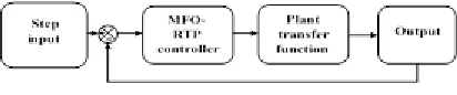
2.7 Experimental Setup

To signify the heat of reaction, an exothermic reaction was preferred. In this reaction, the hydrogen peroxide is decomposed into water and oxygen gas with an iodide catalyst

The reaction involved

2 𝐻 2𝑂 2 (𝑎 𝑞 )−→2𝐻 2𝑂 (𝑙 )+𝑂 2(𝑔 )

The above reaction was used mainly in classrooms to estimate the heat of the reaction and activation energy determined to be -98,000 J/mol. There are several studies that published with hydrogen peroxide decomposition reaction in Journal of Chemical Education. The methods named as ―Efficient Method for the Determination of the Activation Energy of the Iodide-Catalyzed Decomposition of Hydrogen Peroxide were conducted in the lab. In this experimental study, Styrofoam cup calorimeter was taken in which 4mL of 0.10 M potassium iodide mixed to 30mL of 12% hydrogen peroxide. Initial calorimeter experiment was tried to reform the temperature vs time profile established in this study. The temperature increase in the reaction was demonstrated once the heat was removed unknown. Because of the absence of 12% hydrogen peroxide for the experiment, 30% solution was diluted to the required percentage. Then, 30 mL of the 12% solution were included to a calorimeter with the two 8 ounce Styrofoam cups. The experiment is initiated with 4 mL of 0.1 M potassium iodide and it was poured into the cup. The entirety of the run, and the temperature profiles of the container’s inner and outer walls, and also the mixture itself were enclosed in calorimeter and it was note down with the use of type J, bare wire thermocouples. At every second after adding potassium iodide, the data was recorded until the completion of reaction.

Fig. 5 CSTH Photograph

TABLE 5

COMPARISON OF EXISTING AND PROPOSED EXPERIMENTAL PROCEDURE

Hybrid PSO-BFO

BA (Bat Algorithm)

EBA (Enhanced Bat algorithm)

Proposed (MFO)

MSE 0.1578 0.0975 0.089531 0.04785 Undershoot

time 12.7 10.42 6.917 4.178 Rise Time 46.11 40.116 40.0815 30.7072 Settling

Time 250.1109 254.1147 257.9036 426.8621

6829

experimental procedure. The MSE, Undershoot time and Settling time and rise time was achieved better than the other existing algorithms.

3

RESULTS

AND

DISCUSSIONS

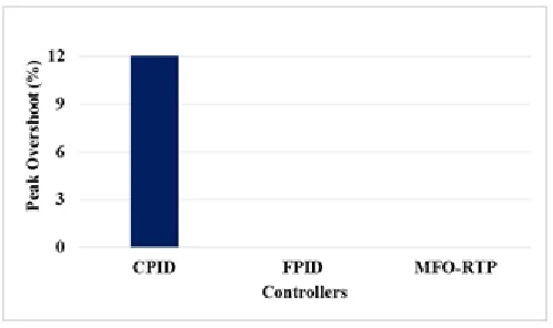
This section analyzes the performance exhibited by the proposed Optimal PID controller that utilizes a Moth-Flame Optimization algorithm for maintaining an optimum level of temperature with in the CSTH. For the specified tank scenario, the transient response inferred is investigated for realizing the distortion of the entire system from an equilibrium to the actual level, where a constant temperature is meant to get maintained. The variations obtained in several transient responses by means of deploying the conventional PID controller, Fuzzy PID controller and the proposed MFO-RTP based controller is exemplified here. The peak overshoot value obtained for acquiring a constant temperature is shown in Fig. 5. The peak overshoot value measured for the employed MFO-PID is of highly minimal value.

Fig. 6. Peak Overshoot analysis

MFO-RTP based controller implements stabilized temperature at the initial stage itself due to the nature of transverse orientation exhibited by moths, an initial moth itself gets diverted toward a best flame i.e., a stable temperature. Hence, the temperature is not necessitated initially to reach a peak overshoot before reaching a stable level of temperature. Total time required for rising the temperature from a minimal level to a required actual level is inferred as rise time. Rise time incurred for various controllers deployed on a CSTH is illustrated in Fig. 7.

Fig. 7. Rise Time analysis

Since the flames are optimized around hyper spheres, the actual temperature is reached without going through manifold exploration stages in a search space. The PID controller that utilizes a fuzzy approach usually undergoes a sequence of updating strategies and hence, the time span incurred to reach a stage of actual temperature is very high. In spite of various positions available, abrupt movement of moths tends to reach a necessitated rise level within no time. Aggregated amount of time suffered to reach an initial level of actual temperature from the initial stage of the process is termed as settling time. The variation realized for various controllers deployed on CSTH is presented in Fig. 8.

Fig. 8. Settling Time analysis

The proposed MFO-RTP based controller is recognized for its minimized settling time and infers a mitigation in reaching the settling time by 89% than other CPID and FPID controllers. The devised MFO-RTP based controller is capable of alleviating the time span in reaching the actual temperature with an enhanced proficiency because of an adaptive convergence of updated flames in accordance with the growth of iterations for which the feasible temperature is searched for. The overall amount of time experienced to traverse form the beginning of the process until the stage of reaching the actual temperature is defined as the delay time and the variations computed on incorporating different controllers is illustrated in Fig. 9.

Fig. 9. Delay Time analysis

6830

archived are retrieved from the matrix and hence, the finest solution flame is opted for reaching actual temperature through the reiteration of the periodical update procedure.

TABLE 6

OUTPUT CHARACTERISTICS INFERRED FOR VARIOUS ALGORITHMS

Algorithm Peak _Overshoot Settling _Time Rise Time

Z-N 7.306 7.5196 2.888

GA 28.21 11.494 1.549

PSO 0.015 7.3931 2.711

GA+PSO 0.016 3.6119 1.022

MFO-RTP 0 0.709 0.5

Among all these algorithms implemented for attaining a constant temperature GA assimilated with PSO algorithm exposes a minimum result of all approaches analyzed (Kantha, Utkarsh, & Kumar, 2014). The peak overshoot value acquired for the proposed MFO-RTP methodology is a null value and other parameters 80%, 51% and 99% for settling time, rise time and delay time respectively.

4

CONCLUSION

This paper discussed the issues involved in deploying a Continuous Stirred Tank Heater to maintain a uniform temperature within an automated system within a complicated scenario is managed. Issues inferred in those conventional approaches in tuning the controller in terms of sustaining the temperature by means of incurring faulty inferences as feedback. Accomplishing a constant temperature is made feasible with the devised MFO-RTP approach. The comparative analysis carried out among the suggested mechanism with the traditional approaches like Zeigler-Nicholos, Genetic Algorithm, Particle Swarm Optimization and a hybrid GA-PSO based tuning evidently proved the proficiency in terms of peak overshoot, settling time, rise time and delay time. Devised MFO-RTP methodology realized a mitigation of about 89 % in settling time and 35 % of delay time.

REFERENCES

[1]. Bhaskarwar, T. V., Giri, S. S., & Jamakar, R. (2015). Automation of shell and tube type heat exchanger with PLC and LabVIEW. Paper presented at the Industrial Instrumentation and Control (ICIC), 2015 International Conference on.

[2]. El-Tantawy, S., Abdulhai, B., & Abdelgawad, H. (2013). Multiagent reinforcement learning for integrated network of adaptive traffic signal controllers (MARLIN-ATSC): methodology and large-scale application on downtown Toronto. IEEE Transactions on Intelligent Transportation Systems, 14(3), 1140-1150.

[3]. He, W., Zi, Y., Chen, B., Wu, F., & He, Z. (2015). Automatic fault feature extraction of mechanical anomaly on induction motor bearing using ensemble super-wavelet transform. Mechanical Systems and Signal Processing, 54, 457-480.

[4]. Heertjes, M. F., Van der Velden, B., & Oomen, T. (2016). Constrained iterative feedback tuning for robust control of a wafer stage system. IEEE

Transactions on Control Systems Technology, 24(1), 56-66.

[5]. Jatoth, R. K., Jain, A. K., & Phanindra, T. (2013). Liquid level control of three tank system using hybrid GA-PSO algorithm. Paper presented at the Engineering (NUiCONE), 2013 Nirma University International Conference on.

[6]. Jouppila, V. T., Gadsden, S. A., Bone, G. M., Ellman, A. U., & Habibi, S. R. (2014). Sliding mode control of a pneumatic muscle actuator system with a PWM strategy. International journal of fluid power, 15(1), 19-31.

[7]. Jung, J.-W., Leu, V. Q., Do, T. D., Kim, E.-K., & Choi, H. H. (2015). Adaptive PID speed control design for permanent magnet synchronous motor drives. IEEE Transactions on Power Electronics, 30(2), 900-908. [8]. Kantha, A. S., Utkarsh, A., & Kumar, J. R. (2014).

Hybrid genetic algorithm-swarm intelligence based tuning of continuously stirred tank reactor. Paper presented at the Industrial and Information Systems (ICIIS), 2014 9th International Conference on. [9]. Léchappé, V., Moulay, E., Plestan, F., Glumineau, A.,

& Chriette, A. (2015). New predictive scheme for the control of LTI systems with input delay and unknown disturbances. Automatica, 52, 179-184.

[10]. Lei, Y., Lin, J., He, Z., & Zuo, M. J. (2013). A review on empirical mode decomposition in fault diagnosis of rotating machinery. Mechanical Systems and Signal Processing, 35(1), 108-126.

[11]. Li, Y., Wang, X., Huang, R., & Qiu, Z. (2015). Active vibration and noise control of vibro-acoustic system by using PID controller. Journal of Sound and Vibration, 348, 57-70.

[12]. Lin, J., & Chen, Q. (2013). Fault diagnosis of rolling bearings based on multifractal detrended fluctuation analysis and Mahalanobis distance criterion. Mechanical Systems and Signal Processing, 38(2), 515-533.

[13]. Ma, X., Jin, J., & Lei, W. (2014). Multi-criteria analysis of optimal signal plans using microscopic traffic models. Transportation Research Part D: Transport and Environment, 32, 1-14.

[14]. Marino, H., Bergeles, C., & Nelson, B. J. (2014). Robust electromagnetic control of microrobots under force and localization uncertainties. IEEE

Transactions on Automation Science and

Engineering, 11(1), 310-316.

[15]. Ouyang, P. R., Pano, V., & Dam, T. (2015). PID position domain control for contour tracking. International Journal of Systems Science, 46(1), 111-124.

[16]. Pi, Q., & Ye, H. (2015). Survey of particle swarm optimization algorithm and its applications in antenna circuit. Paper presented at the Communication Problem-Solving (ICCP), 2015 IEEE International Conference on.

[17]. Rojjananil, K., & Assawinchaichote, W. (2016). Optimized PIDI 2 D 2 Controller Based on Genetic Algorithm for Three-tank Liquid Level Control System. Procedia Computer Science, 86, 100-103. [18]. Sabir, M. M., & Ali, T. (2016). Optimal PID controller

6831

Computation, 274, 690-699.

[19]. Sahib, M. A., & Ahmed, B. S. (2016). A new multiobjective performance criterion used in PID tuning optimization algorithms. Journal of advanced research, 7(1), 125-134.

[20]. Salazar, M., & Méndez, F. (2014). PID control for a single-stage transcritical CO 2 refrigeration cycle. Applied Thermal Engineering, 67(1), 429-438. [21]. Shah, P., & Agashe, S. (2016). Review of fractional

PID controller. Mechatronics, 38, 29-41.

[22]. Sharma, M., Verma, P., & Mathew, L. (2016). Design an intelligent controller for a process control system. Paper presented at the Innovation and Challenges in

Cyber Security (ICICCS-INBUSH), 2016

International Conference on.

[23]. Shi, R., He, T., Peng, J., Zhang, Y., & Zhuge, W. (2016). System design and control for waste heat recovery of automotive engines based on Organic Rankine Cycle. Energy, 102, 276-286.

[24]. Tepljakov, A., Gonzalez, E. A., Petlenkov, E., Belikov, J., Monje, C. A., & Petráš, I. (2016). Incorporation of fractional-order dynamics into an existing PI/PID DC motor control loop. ISA transactions, 60, 262-273. [25]. Xu, Y., Zhou, J., Xue, X., Fu, W., Zhu, W., & Li, C.