ISSN (e): 2250-3021, ISSN (p): 2278-8719 Vol. 04, Issue 08 (August. 2014), ||V4|| PP 18-32
Analysis on Variable Fluid Viscosity of Non-Darcian Flow over a
Moving Vertical Plate in a Porous Medium with Suction and
Viscous Dissipation
Animasaun, I. L.
1and Aluko, O. B.
21
Mathematical Science Department, Federal University of Technology, Akure, Nigeria.
2
Mathematics/Statistics Department, Osun State Polytechnic, Iree, Nigeria.
Abstract: - An analysis is carried out to study free convective flow and heat transfer of a viscous incompressible fluid over a linearly moving vertical porous plate with suction and viscous dissipation. The fluid viscosity is assumed to vary as a linear function of temperature. The governing boundary layer equations are reduced to boundary value problem using the concept of similarity transformations. The corresponding coupled ordinary differential equation is solved numerically using the Runge Kutta fourth order method along with shooting technique. Graphical results for the dimensionless velocity and temperature distributions are shown for various values of the thermophysical parameters controlling the flow regime. Numerical values of physical quantities such as the local Skin-friction coefficient and the Local Nusselt number are presented in tabular form.
Keywords: -Variable fluid viscosity, Porous media, Viscous Dissipation, Non Darcian flow, Radiative Heat flux
I. INTRODUCTION
The physics of fluid flow in different media and conduits is a well-researched area in engineering with groundbreaking works by pioneer workers in the field of engineering. Likewise, transportation of heat through porous media has gained considerable attention due to its vast applications in the industry and also due to the increasing need for a better understanding of the associated transport processes. There are numerous practical applications in the industry which can be modeled or can be approximated as transport through porous media such as grain storage, heat exchanger devices, petroleum reservoirs, chemical catalytic reactors and processes, geothermal and geophysical engineering, moisture migration in a fibrous insulation and nuclear waste disposal and others. Bejan and Khair [2] investigated the free convection boundary layer flow in a porous medium owing to combined heat and mass transfer. Lai and Kulacki [8] used the series expansion method to investigate coupled heat and mass transfer in natural convection from a sphere in a porous medium. The suction and blowing effects on free convection coupled heat and mass transfer over a vertical plate in a saturated porous medium were studied by Raptis et al. [18]. The analysis of convective transport in a porous medium with the inclusion of non-Darcian effects has also been a matter of study in recent years. The inertia effect is expected to be important at a higher flow rate and it can be accounted for through the addition of a velocity squared term in the momentum equation, which is known as the Forchheimer’s extension of the Darcy’s law. A detailed review of convective heat transfer in Darcy and non-Darcy porous medium can be found in the book by Nield and Bejan [14]. The problem of flow and heat transfer in a laminar boundary layer over a stretching sheet in a saturated porous medium has an important application in the metallurgy and chemical engineering fields. Layek
et al. [7] considered the flow and heat transfer boundary layer stagnation point flow of an incompressible viscous fluid towards a heated porous stretching sheet embedded in a porous medium subject to suction/blowing with internal heat generation or absorption.
Sakiadis in 1961 was the first person to study the laminar boundary layer flow caused by a rigid surface moving in its own plane. Crane in 1970 extended the work of Sakiadis by considering the same model subject to stretching plate. Gupta and Gupta [6]studied the problem in the light of suction or blowing. Recently, Prasanna
et al. [17] studied MHD Boundary Layer Flow of Heat and Mass Transfer over a Moving Vertical Plate in a Porous Medium with Suction and Viscous Dissipation; the governing boundary layer equations are reduced to a two-point boundary value problem using similarity transformations. The resultant problem is solved numerically using the Runge-Kutta fourth order method along with shooting technique. The momentum boundary layer thickness decreases, while both thermal and concentration boundary layer thicknesses increase with an increase in the magnetic field intensity. All the above mentioned investigations were carried out for fluids having constant viscosity throughout the boundary-layer. However it is known that these physical properties may change significantly with temperature. For instance, the viscosity of water decreases about 240% when the temperature increases from (100c)to (500 ).
c The viscosity of air is 0.6924105,
1
.
3289
,
2
.
286
and625 .
predict accurately the flow behaviors in the boundary layer, it is necessary to take the variation of viscosity into account. The study of viscous incompressible fluid flow with temperature dependent properties is of great importance in industries such as food processing, coating and polymer processing where temperature is generated. In industrial systems, fluid flow can be subjected to extreme conditions such as high temperature, pressure, and shear rates. In addition, external heating such as the ambient temperature and high shear rates can lead to a high temperature being generated within the fluid. All these conditions normally have a significant effect on the fluid properties. In fluid dynamics, it is well known that the property which is most sensitive to temperature rise is viscosity. Fluids used in industries such as polymer fluids, engine oil, palm oil have a viscosity that varies rapidly with temperature and this eventually give rise to strong feedback effects which normally lead to significant changes in the structure of the fluid flow, Wyle and Huang [21]. Mukhopadhyay et al. [12] carried out a comprehensive research on free convective boundary layer flow and heat transfer of a fluid with variable viscosity over a porous stretching vertical surface in presence of thermal radiation, Lie group transformation was adopted and fourth order classical Runge Kutta method was adopted to solve the corresponding coupled ordinary differential equations. They reported that; with an increase of temperature dependent fluid viscosity parameter, the fluid velocity increases but the temperature decreases at a particular point of the sheet. In the present research, we study free convective flow and radiative heat transfer of viscous incompressible fluid having variable viscosity over a stretching porous vertical plate which is an extension of Mukhopadhyay et al. [12]. We further assume that the fluid flow is under the influence of viscous dissipation and Darcy-Forchheimer. The basic equations governing the flow field are partial differential equations and these have been reduced to a set of ordinary differential equations by applying suitable similarity transformations. The resultant equations are coupled and non-linear, and hence are solved numerically using the fourth order Runge-Kutta method along with shooting technique. The effects of various governing parameters on the velocity and temperature are presented graphically and discussed quantitatively.
II. MATHEMATICALFORMULATION
A steady two-dimensional laminar free convection flow of a viscous incompressible electrically conducting fluid along a porous vertical stretching sheet, in the presence of suction and viscous dissipation, is considered. The
x
axis is taken along the plate in the upward direction and they
axis is normal to the sheet. The velocity of the fluid far away from the plate surface is assumed to be zero. Assuming that the Boussinesq’s and boundary layer approximation hold and using the Darcy-Forchheimer model, the basic equations which govern the problem are given by (Mukhopadhyay et al. [12] and Prasanna et al. [16] ) and reformulated as:0
y
v
x
u
(1)
2 *
2 2
1
)
(
)
(
)
(
)
(
1
u
K
b
u
K
T
T
T
g
y
u
T
y
u
y
T
T
T
y
u
v
x
u
u
(2)2
2 2
)
(
)
(
1
y
u
C
T
T
T
C
q
y
q
C
y
T
C
y
T
v
x
T
u
P P
r
P
P
(3)
Subject to boundary conditions
m
Bx
u
v
V
T
T
W aty
0
(4a)0
u
T
T
asy
(4b)The heat transfer of viscous incompressible fluid flow over a vertical stretching sheet emerging out of a slit at origin
(
x
0
,
y
0
)
., The viscous dissipation term in the energy equation is significant (we assumed that the fluid velocity is high),
x
andy
represent coordinate axes along the continuous surface in the direction of motion and perpendicular to it, respectively,u
andv
are the Darcian velocity components alongx
andy
directions,
Density (assumed constant),g
is the gravity,b
* is the empirical constant,
is the viscosity,
(
T
)
is the kinematic viscosity,B
T is the coefficients of thermal expansion,K
is the permeabilityof the porous medium,
is the thermal conductivity,C
P is the specific heat at constant pressure,q
Dimensional heat absorption coefficient. Using (Brewster [3]), radiative heat flux
q
r is described by they
T
k
q
r
4 *3
4
(5)where
is the Stefan-Boltzmann constant andk
* is known as the absorption coefficient. Assuming that thetemperature difference within the flow is such that
T
4 may be expanded in a Taylor series and expandingT
4about
T
and neglecting higher orders. It is assumed that the temperature differences within the flow aresufficiently small such that
T
4 can be expressed as a linear function of temperature. This is accomplished by expandingT
4 in a Taylor series about the free stream temperatureT
4 and neglecting higher-order terms. The Taylor’s series expansion of a functionf
(
x
)
aboutx
0
)
(
!
...
)
(
''
!
2
)
(
)
(
)
(
)
(
0 00 2 0 0 ' 0
0
f
x
n
x
x
x
f
x
x
x
f
x
x
x
f
x
f
n n
...
!
2
)
(
)
(
2 42 2 4
4
4
T
dT
d
T
T
T
dT
d
T
T
T
T
4 3 43
4
TT
T
T
(6)3 4 4 T T T (7)
Making use of (5) and (7), equation (3) becomes
2
2 2
* 3
1
(
)
)
(
3
16
y
u
C
T
T
T
C
q
y
T
C
k
T
C
y
T
v
x
T
u
P P P P
(8)We now introduce the following relations for
u
,
v
,
and
,
y
u
x
v
and
T
T
T
T
W
(9)2 * 2 2
1
)
(
)
(
)
(
)
(
1
y
K
b
y
K
T
T
T
g
y
y
T
y
y
y
T
T
T
y
y
x
y
x
y
2 2 2 * 31
(
)
3
16
y
y
C
T
T
C
q
y
T
C
k
T
C
y
T
x
x
T
y
P P P P
where
u
is the stream function. The streamwise velocity and the suction velocity are taken asm
Bx
x
U
(
)
andv
V
. In this research,m
is the power law exponent,m
1
/
2
,B
0
,
T
Wis thewall temperature and
T
is the ambient temperature, the fluid viscosity
is assumed to vary as a linear function of temperature. According to Batchelor [1],)]
(
[
)
(
T
*a
b
T
W
T
(10) where
* is the constant value of the coefficient of viscosity far from the sheet (reference viscosity) anda
,
b
are constants
(
b
0
)
. In this research, we consider the case whena
1
For a viscous fluid, Ling and Dybbs[9]suggest a viscosity dependence on temperature
T
of the form
1
(
T
T
)
1 , where
is a thermal property of the fluid and
is the viscosity away from the hot sheet. Others temperature dependent viscosity model are Reynold’s model
(
T
)
0exp(
M
(
T
T
0))
and Vogel’s model
0 0exp
)
(
T
b
a
T
(see e.g., Massoudi and Christe [11], Nadeem and Ali [13], Okoya [15]) and Pardemirli and Yilbas [16]. Our adopted model (10) does not differ at all with all the model mentioned above. The range of temperature, i.e.
T
)
)(
1
(
T
T
T
T
W
WUsing (10) above relations in the boundary layer equation (2) and in the modified energy equation (8), we get
)
(
]
)
1
(
[
3 3 * 2 2 *
T
T
g
y
a
y
y
y
y
x
y
x
y
W
2 * *]
)
1
(
[
y
K
b
y
K
a
(11) 2 2 * 31
(
)
3
16
y
T
T
C
k
T
C
y
T
x
x
T
y
P P W
2 *]
)
1
(
[
)
(
y
y
C
a
T
T
C
q
P W P
(12)where
b
(
T
W
T
)
, Subject tom
Bx
y
V
x
1
aty
0
(13)0
y
1
asy
(14)To transform equations (11)-(14) into a set of ordinary differential equations, the following similarity transformations and dimensionless variables are introduced
4 1
yx
4 *(
)
3
x
f
b
g
J
Gr 2 *4
x
b
F
S *
2x
K
D
a
K
x
k
2 1 24
3 1 *4
T
k
N
p rC
P
P
C
q
x
* 21
4
)
(
4
* 2
T
T
C
x
E
W P c
S
x
*V
4 1
3
4
where
f
(
),
(
),
,
F
S,D
a,k
2,
N
,
P
r,
,
E
c,
S
andJ
Grare dimensionless stream function, dimensionless temperature, similarity variable, Local Forchhemier parameter, Local Darcy Parameter, Permeability related parameter of the porous medium, Radiation parameter, Prandtl number, Heat generation/Absorption parameter, Eckert related Parameter, Suction parameter and Grashof related parameter respectively. It is known thatr Gr
G
J
(Local Grashof number), in this research.0
4
]
)
1
(
[
4
3
2
]
)
1
(
[
4
2 2 2 2 2 2 2 3 3
d
df
D
F
d
df
a
k
J
d
f
d
d
d
d
f
d
f
d
df
d
f
d
a
a s Gr (15)0
]
)
1
(
[
3
3
4
1
4
2 2 2 2 2
d
f
d
a
E
P
P
d
d
f
P
d
d
N
r r r c (16)Subject to *
B
d
df
f
S
1
at
0
(17)0
d
df
0
as
(18)III. NUMERICALSOLUTION
simultaneous differential equations of first order and they are further transformed into initial value problem by applying the shooting technique. The resultant initial value problem is solved by employing Runge-Kutta fourth order technique. The step size
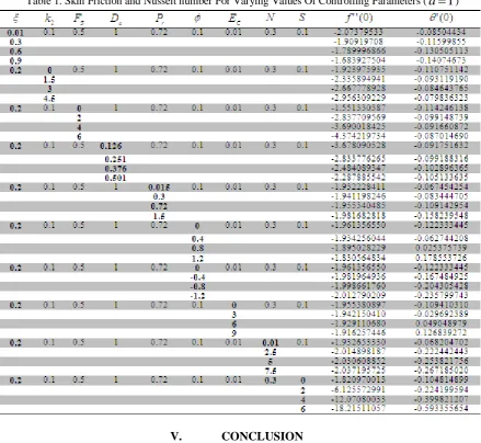
0.05 is used to obtain the numerical solution with fifteen decimal place accuracy as the criterion of convergence. From the process of numerical computation, the skin-friction coefficient, and the Nusselt number, which are respectively proportional tof
'
'
(
0
)
and
'
(
0
)
are also sorted out and their numerical values are presented in a tabular form.IV. FIGURESANDDISCUSSIONS
The effect of Local Forchheimer parameter, permeability parameter, Radiation parameter, Prandtl number, Heat generation/Absorption parameter, Eckert Number and Suction parameter has been formulated and solved numerically. In order to understand the flow of the fluid, computations are performed for different
parameters such as
,
F
S,D
a,k
2,
N
,
P
r,
,
E
c,
S
.In this research,*
B
,a
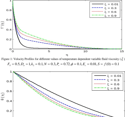
and JGr is chosen to be equal toone. Figure 1 exhibit the velocity profiles for several values of
with Pr 0.72 in the presence of suction1
.
0
S
whenN 0.3. In the case of uniform suction, the velocity of the fluid is found to increase with theincrease of the temperature dependent fluid viscosity parameter
. This can be explained physically as theparameter
increases, the bond between the fluids becomes weaker and the viscosity decrease and the fluidflow at faster rate. In Figure 2, variations of temperature field
(
)
with
for several values of
using01
.
0
,
1
.
0
,
72
.
0
,
3
.
0
,
1
.
0
,
1
,
5
.
0
2
a r cS
D
k
N
P
E
F
in the presence of suction(
S
f
(
0
)
0
.
1
) are shown. It is observed that the temperature decreases with the increasing values of
. The increase of temperature dependent fluid viscosity parameter leads to decrease of thermal boundary layer thickness, which results in decrease of temperature profile
(
)
. Decrease in temperature profiles across the thermal boundary layer means a decrease in the velocity of the fluid properties(
)
. As a matter of fact, in this case, the fluid particles undergo two opposite forces which are: (i) One force increases the fluid velocity due to decrease in the fluid viscosity with increase in the values of
,
(ii) The second force decreases the fluid velocity due to decrease in temperature. {Since
(
)
decreases with increasing
}.Very near the vertical surface0
0
.
2
, as the temperature
(
)
is high, the first force dominates and far away from the surface,15
1
.
14
, the temperature
(
)
is low; this implies that the second force dominates in that region.Figure 3 illustrates the effect of permeability parameter
(
k
2)
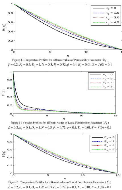
on the velocity. It is noticed that as thepermeability parameter increases, the velocity decreases. Since the porosity of the plate increases, as the fluid flows over the porous plate, the drag tends to increase which draw back the velocity. Also, Figure 4 shows the variation of the thermal boundary-layer with the effects of permeability parameter
(
k
2)
. We noticed that the thermal boundary layer thickness increases with an increase in the permeability parameter. Physically, this can be explained as follows, as the porosity parameter increases, this give rooms to more entrance of heat into the flow. As the heat increases, the temperature profiles also become affected and tend to increase. Figure 5 and Figure 6 reveal that the effect of Forchhemier parameter is experienced near the plate only, increase in the value ofF
S leads to decrease in velocity within0
6
.
1
.
Reverse is the case on temperature profiles, asForchhemier parameter
F
S increases, the temperature
(
)
increases throughout the flow region. We chose501
.
0
,
376
.
0
,
251
.
0
,
126
.
0
a
D
and high value of Forchhemier number (F
S
0
.
5
) to analyze the effectof the local Darcy number
D
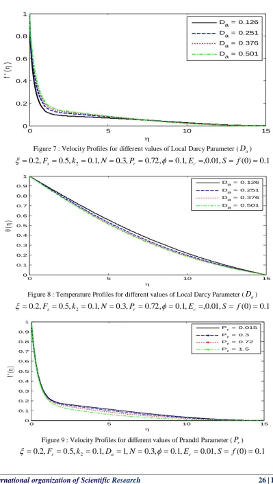
a on the velocity profiles and temperature fields as shown in Figure 7 and 8.Figure 7 depicts that the velocity increases slightly with an increase in the values of
D
a. The effect of localDarcy number is experienced within a certain range, increase in the value of
D
a leads to increase in velocitywithin
0
6
.
5
. Reverse is the case on temperature profiles, asD
a increases, the temperature
(
)
decreases slightly. The decrease in
(
)
across the flow region is of slower rate. This effect is negligible on the temperature due to the distinction of the values of Da. On the velocity profiles, effect ofD
a is negligible farPrandtl number (Mercury with
P
r
0
.
015
) are much more responsive to thermal radiation than fluids (Air withP
r
0
.
72
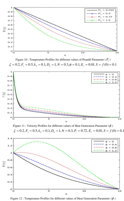
) having a larger Prandtl number. It is also noted from figures 9 and 10 that temperature andvelocity decreases with the increasing value of Prandtl number. From figure 9, effects of
P
ris negligible very close to the wall0
0
.
9
and far from the wall13
.
32
15
We have illustrated non-dimensional velocity, temperature against
for some representative values ofthe heat source/absorption parameter
0
,
0
.
4
,
0
.
8
,
1
.
2
,
positive value of
represents source i.e. heat generation in the fluid while negative value of
represents absorption of the heat that exists within the fluid.Figure 11 and 12 shows effect of heat source parameter
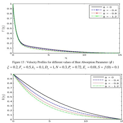
over velocity and temperature profiles. It is observed that, due to the generation of heat into the fluid flow; the buoyancy force increases which in turn gives higher velocity in the velocity and thermal boundary layer. Also, Figure 13 and 14 shows effect of heat absorption parameter
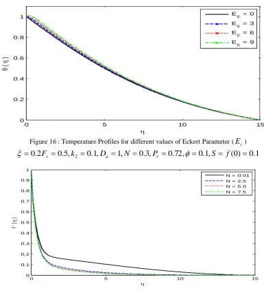
over velocity and temperature profiles, due to the absorption of heat from the fluid flow; the buoyancy force decreases which in turn gives lower velocity in the velocity and thermal boundary layer. Figure 15 shows the variation of Eckert number (E
c) over the momentum boundary-layer, we observed thatE
c does not have any substantial effect on velocity of the fluid flow. Also, Fig 16 shows the variation of the thermal boundary-layer with the Eckert number (E
c). It is observed that the thermal boundary layer thickness increasesslightly with an increase in the Eckert number (
E
c). The variation of velocity, and temperature distributionswith radiation parameter N are shown in Figure 17 and 18 respectively. From Figure 17 and 18, we observe that the velocity and the temperature profiles decrease with the increase of radiation parameter
N
. Radiation can be used to control the velocity and the thermal boundary layers quite effectively. The effect of radiation parameterN
on the velocity boundary layer is shown in Figure 17 for1
.
0
)
0
(
,
01
.
0
,
1
.
0
,
72
.
0
,
1
,
1
.
0
,
5
.
0
,
2
.
0
2
F
sk
D
aP
r
E
cS
f
.The velocity profilesshow a decrease far from the plate with the increase of radiation parameter
N
. It is noted from Figure 18 that the temperature decreases with the increasing value of the radiation parameterN
. The effect of radiation parameterN
is to reduce the temperature significantly in the flow region. The increase in radiation parameter means the release of heat energy from the flow region and so the fluid temperature decreases as the thermal boundary layer thickness becomes thinner. This result can be further explained by the fact that a decrease in thevalue of 3
1 *
4
/
k T
N for a given k* and T means a decrease in the Roseland radiation absorptivity.
According to momentum and energy equations, the divergence of the radiative heat flux qr /y increases as
k
decreases which in turn increases the rate of radiative heat transferred to the fluid and hence the fluid temperature increases. In view of this explanation, the effect of radiation becomes more significant as0
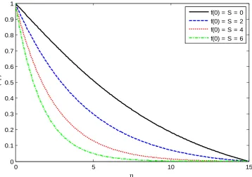
N (N 0) and can be neglected when N . Figure 19 and 20 represents the effects of suction on fluid velocity and temperature when the fluid viscosity is uniform 0. With an increase in the value of
0 5 10 15 0
0.2 0.4 0.6 0.8 1
f '
(
)
= 0.01
= 0.3
= 0.6
= 0.9
Figure 1: Velocity Profiles for different values of temperature dependent variable fluid viscosity (
)1
.
0
)
0
(
,
01
.
0
,
1
.
0
,
72
.
0
,
3
.
0
,
1
.
0
,
1
,
5
.
0
2
D
k
N
P
E
S
f
F
S a r
c0 5 10 15
0 0.2 0.4 0.6 0.8 1
(
)
= 0.01
= 0.3
= 0.6
= 0.9
Figure 2 : Temperature Profiles for different values of temperature dependent variable fluid viscosity (
)1
.
0
)
0
(
,
01
.
0
,
1
.
0
,
72
.
0
,
3
.
0
,
1
.
0
,
1
,
5
.
0
2
D
k
N
P
E
S
f
F
S a r
c0 5 10 15
0 0.2 0.4 0.6 0.8 1
f '
(
)
k2 = 0
k2 = 1.5
k2 = 3.0
k2 = 4.5
Figure 3 : Velocity Profiles for different values of Permeability Parameter (
k
2)1
.
0
)
0
(
,
01
.
0
,
1
.
0
,
72
.
0
,
3
.
0
,
1
,
5
.
0
,
2
.
0
F
SD
aN
P
r
E
cS
f
0 5 10 15 0
0.2 0.4 0.6 0.8 1
(
)
k2 = 0
k
2 = 1.5 k
2 = 3.0 k
2 = 4.5
Figure 4 : Temperature Profiles for different values of Permeability Parameter (
k
2)1
.
0
)
0
(
,
01
.
0
,
1
.
0
,
72
.
0
,
3
.
0
,
1
,
5
.
0
,
2
.
0
F
SD
aN
P
r
E
cS
f
0 5 10 15
0 0.2 0.4 0.6 0.8 1
f '
(
)
Fs = 0
Fs = 2
F
s = 4
Fs = 6
Figure 5 : Velocity Profiles for different values of Local Forchheimer Parameter (
F
S)1
.
0
)
0
(
,
01
.
0
,
1
.
0
,
72
.
0
,
3
.
0
,
1
,
1
.
0
,
2
.
0
2
k
D
aN
P
r
E
cS
f
0 5 10 15
0 0.2 0.4 0.6 0.8 1
(
)
Fs = 0
Fs = 2
F
s = 4
F
s = 6
Figure 6 : Temperature Profiles for different values of Local Forchheimer Parameter (
F
S)1
.
0
)
0
(
,
01
.
0
,
1
.
0
,
72
.
0
,
3
.
0
,
1
,
1
.
0
,
2
.
0
2
k
D
aN
P
r
E
cS
f
0 5 10 15 0
0.2 0.4 0.6 0.8 1
f '
(
)
Da = 0.126 Da = 0.251 Da = 0.376 Da = 0.501
Figure 7 : Velocity Profiles for different values of Local Darcy Parameter (
D
a)1
.
0
)
0
(
,
01
.
0
,
,
1
.
0
,
72
.
0
,
3
.
0
,
1
.
0
,
5
.
0
,
2
.
0
2
F
sk
N
P
r
E
cS
f
0 5 10 15
0 0.1 0.2 0.3 0.4 0.5 0.6 0.7 0.8 0.9 1
(
)
Da = 0.126
Da = 0.251
Da = 0.376
Da = 0.501
Figure 8 : Temperature Profiles for different values of Local Darcy Parameter (
D
a)1
.
0
)
0
(
,
01
.
0
,
,
1
.
0
,
72
.
0
,
3
.
0
,
1
.
0
,
5
.
0
,
2
.
0
2
F
sk
N
P
r
E
cS
f
0 5 10 15
0 0.1 0.2 0.3 0.4 0.5 0.6 0.7 0.8 0.9 1
f '
(
)
Pr = 0.015 Pr = 0.3 Pr = 0.72 Pr = 1.5
Figure 9 : Velocity Profiles for different values of Prandtl Parameter (
P
r)1
.
0
)
0
(
,
01
.
0
,
1
.
0
,
3
.
0
,
1
,
1
.
0
,
5
.
0
,
2
.
0
2
F
sk
D
aN
E
cS
f
0 5 10 15 0
0.1 0.2 0.3 0.4 0.5 0.6 0.7 0.8 0.9 1
(
)
Pr = 0.015
Pr = 0.3
Pr = 0.72
Pr = 1.5
Figure 10 : Temperature Profiles for different values of Prandtl Parameter (
P
r)1
.
0
)
0
(
,
01
.
0
,
1
.
0
,
3
.
0
,
1
,
1
.
0
,
5
.
0
,
2
.
0
2
F
sk
D
aN
E
cS
f
0 5 10 15
0 0.1 0.2 0.3 0.4 0.5 0.6 0.7 0.8 0.9 1
f '
(
)
= 0
= 0.4
= 0.8
= 1.2
Figure 11 : Velocity Profiles for different values of Heat Generation Parameter (
)
0
.
2
,
F
s
0
.
5
,
k
2
0
.
1
,
D
a
1
,
N
0
.
3
,
P
r
0
.
72
,
E
c
0
.
01
,
S
f
(
0
)
0
.
1
0 5 10 15
0 0.2 0.4 0.6 0.8 1 1.2 1.4
(
)
= 0
= 0.4
= 0.8
= 1.2
Figure 12 : Temperature Profiles for different values of Heat Generation Parameter (
)1
.
0
)
0
(
,
01
.
0
,
72
.
0
,
3
.
0
,
1
,
1
.
0
,
5
.
0
,
2
.
0
2
F
sk
D
aN
P
rE
cS
f
0 5 10 15 0
0.1 0.2 0.3 0.4 0.5 0.6 0.7 0.8 0.9 1
f '
(
)
= 0
= - 0.4
= - 0.8
= - 1.2
Figure 13 : Velocity Profiles for different values of Heat Absorption Parameter (
)1
.
0
)
0
(
,
01
.
0
,
72
.
0
,
3
.
0
,
1
,
1
.
0
,
5
.
0
,
2
.
0
2
F
sk
D
aN
P
rE
cS
f
0 5 10 15
0 0.1 0.2 0.3 0.4 0.5 0.6 0.7 0.8 0.9 1
(
)
= 0
= - 0.4
= - 0.8
= - 1.2
Figure 14 : Temperature Profiles for different values of Heat Absorption Parameter (
)1
.
0
)
0
(
,
01
.
0
,
72
.
0
,
3
.
0
,
1
,
1
.
0
,
5
.
0
,
2
.
0
2
F
sk
D
aN
P
rE
cS
f
0 5 10 15
0 0.1 0.2 0.3 0.4 0.5 0.6 0.7 0.8 0.9 1
f '
(
)
Ec = 0
Ec = 3
Ec = 6
E c = 9
Figure 15 : Velocity Profiles for different values of Eckert Parameter (
E
c)1
.
0
)
0
(
,
1
.
0
,
72
.
0
,
3
.
0
,
1
,
1
.
0
,
5
.
0
2
.
0
2
F
sk
D
aN
P
r
S
f
0 5 10 15 0
0.2 0.4 0.6 0.8 1
(
)
Ec = 0
Ec = 3
Ec = 6
Ec = 9
Figure 16 : Temperature Profiles for different values of Eckert Parameter (
E
c)1
.
0
)
0
(
,
1
.
0
,
72
.
0
,
3
.
0
,
1
,
1
.
0
,
5
.
0
2
.
0
2
F
sk
D
aN
P
r
S
f
0 5 10 15
0 0.1 0.2 0.3 0.4 0.5 0.6 0.7 0.8 0.9 1
f '
(
)
N = 0.01 N = 2.5 N = 5.0 N = 7.5
Figure 17 : Velocity Profiles for different values of Radiation Parameter (
N
)1
.
0
)
0
(
,
01
.
0
,
1
.
0
,
72
.
0
,
1
,
1
.
0
,
5
.
0
,
2
.
0
2
F
sk
D
aP
r
E
cS
f
0 5 10 15
0 0.1 0.2 0.3 0.4 0.5 0.6 0.7 0.8 0.9 1
(
)
N = 0.01 N = 2.5 N = 5.0 N = 7.5
Figure 18 : Temperature Profiles for different values of Radiation Parameter (
N
)1
.
0
)
0
(
,
01
.
0
,
1
.
0
,
72
.
0
,
1
,
1
.
0
,
5
.
0
,
2
.
0
2
F
sk
D
aP
r
E
cS
f
0 5 10 15 0
0.1 0.2 0.3 0.4 0.5 0.6 0.7 0.8 0.9 1
f
'
(
)
f(0) = S = 0 f(0) = S = 2 f(0) = S = 4 f(0) = S = 6
Figure 19 : Velocity Profiles for different values of Suction Parameter (
S
),
01
.
0
,
1
.
0
,
72
.
0
,
3
.
0
,
1
,
1
.
0
,
5
.
0
,
2
.
0
2
F
sk
D
aN
P
r
E
c
0 5 10 15
0 0.1 0.2 0.3 0.4 0.5 0.6 0.7 0.8 0.9 1
(
)
f(0) = S = 0 f(0) = S = 2 f(0) = S = 4 f(0) = S = 6
Figure 20: Temperature Profiles for different values of Suction Parameter (
S
),
01
.
0
,
1
.
0
,
72
.
0
,
3
.
0
,
1
,
1
.
0
,
5
.
0
,
2
.
0
2
F
sk
D
aN
P
r
E
cTable 1. Skin Friction and Nusselt number For Varying Values Of Controlling Parameters (
a
1
)V. CONCLUSION
In this paper, a boundary layer analysis for natural convection heat transfer of a variable viscosity, incompressible fluid over a linearly moving porous vertical surface is considered. From the numerical results pertaining to the present study indicates that the effect of increasing temperature dependent fluid viscosity parameter on a viscous incompressible fluid is to increase the flow velocity which in turn causes the temperature to decrease. The higher values of the Forchheimer number (Fs) indicate lower velocity very close to the wall
but negligible far from the wall and also indicate significant increase of temperature across the flow region. Velocity profiles increase with the increasing value of Darcy number (Da). Magnetic field retards the motion of
the fluid and suction stabilizes the hydrodynamic and thermal boundary layers growth. Horizontal velocity
) ( '
f and temperature ()decreases with the increase in Prandtl parameter and radiation parameter.
VI. ACKNOWLEDGEMENTS
One of the authors (Animasaun, I. L.) gratefully acknowledge the support of Prof. O. K. Koriko, Dr. E. A. Adebile and Dr. A. J. Omowaye for their investment both directly and indirectly on this work.
REFERENCES
[1] Batchelor, G.K. (1987). An Introduction to Fluid Dynamics, Cambridge University Press, London. [2] Bejan, A. and Khair, K.R. (1985). Heat and mass transfer by natural convection in a porous medium, Int.
J. Heat Mass Transfer, Vol. 28, pp.909-918.
[3] Brewster,M. Q. (1972). Thermal Radiative Transfer Properties, John Wiley and Sons, Chichester. [4] Cebeci, T. and Bradshaw, P. (1984). Physical and Computational Aspects of Convective Heat Transfer,
New York, Springer.
[6] Gupta, P.S. and Gupta, A.S. (1977). Heat and mass transfer on a stretching sheet with suction and blowing, Can. J. Chem. Eng. 55,744–746.
[7] Layek, G. C. (2007). Mukhopadhyay S. and Samad S. K. , Int. Comm. Heat Mass Trans. 34, 347.
[8] Lai F.C. and Kulacki F.A. (1990). Coupled heat and mass transfer from a sphere buried in an infinite porous medium, Int. J. Heat Mass Transfer, Vol. 33, pp.209-215.
[9] Ling, J.X. and Dybbs, A. (1987). Forced convection over a flat plate submersed in a porous medium: variable viscosity case, American Society of Mechanical Engineers, NY, Paper 87-WA/HT-23.
[10] Loganathan, P. and Arasu, P.P. (2010). Lie Group Analysis for the Effects of Variable Fluid Viscosity and Thermal Radiation on Free Convective Heat and Mass Transfer with Variable Stream Condition,
Scientific Research Journal, Vol 2, 625-634. doi:10.4236/eng.2010.28080
[11] Massoudi, M. and Christe, I. (1995). Effects of variable viscosity and viscous dissipation on the flow of third grade fluid in a pipe, Int. J. Non-Linear Mech. 30 (5) 687-699.
[12] Mukhopadhyay, S. and Layek, G.C. (2008). Effects of thermal radiation and variable fluid viscosity on free convective flow and heat transfer past a porous stretching surface, International Journal of Heat and Mass Transfer. 51,2167-2178
[13] Nadeem, S. and Ali, M. (2009). Analytical solutions for pipe flow of a fourth grade fluid with Reynold and Vogel’s models of viscosities, Communications in Nonlinear Science and Numerical Simulation, 14 (5) 2073-2090.
[14] Nield, D.A. and Bejan, A.(2006). Convection in Porous Media, Springer-Verlag, New York.
[15] Okoya, S. S.(2011). Disappearance of criticality for reactive third - grade fluid with Reynold’s model viscosity in a flat channel, Int. J. Non-Linear Mechanics, 46 (9) 1110-1115.
[16] Pakdemirli, M. and Yilbas, B. S. (2006). Entropy generation for pipe flow of a third grade fluid with Vogel model viscosity, Int. J. Non-Linear Mechanics 41 (3) 432-437.
[17] Prasanna, M. L., Bhaskar, N. R. and Poornima, T. (2012). MHD Boundary Layer Flow of Heat and Mass Transfer over a moving Vertical Plate in a Porous Medium with Suction and Dissipation, International Journal of Engineering Research and Applications (IJERA), Vol.2, Issue 5, pp. 149-159, ISSN: 2248-9622.
[18] Raptis A., Tzivanidis G. and Kafousias N. (1981). Free convection and mass transfer flow through a porous medium bounded by an infinite vertical limiting surface with constant suction, Letter, Heat Mass Transfer, Vol.8, pp.417-424.
[19] Sakiadis, B.C. (1961) . Boundary-layer behaviour on continuous solid surface: I. The boundary-layer equations for two dimensional and asymmetric flow, AIChE J. 7,26.
[20] Sakiadis, B.C. (1961). Boundary-layer behaviour on continuous solid surface: II. The boundary-layer on a continuous flat surface, AIChE J. 7, 221.