A Hybrid Forecasting Model Based On
Automatic Clustering Algorithm And Fuzzy Time
Series
Nghiem Van Tinh
Thai Nguyen University of Technology, Thai Nguyen University
Thai Nguyen, Vietnam
Nguyen Thi Phuong Nhung
Thai Nguyen University of Technology, Thai Nguyen University
Thai Nguyen, Vietnam
Abstract—In our daily life, people often use forecasting techniques to forecast real problems, such as forecasting stock market, forecasting enrolments, temperature prediction, population growth prediction, etc. In recent years, many researchers used fuzzy time series to handle prediction problems. When forecasting these problems based on fuzzy time series, it is obvious that the length of intervals in the universe of discourse is important because it can affect the forecasting accuracy rate. However, some of the existing fuzzy forecasting methods based on fuzzy time series used the static length of intervals, i.e., the same length of intervals. The disadvantage of the static length of intervals is that the historical data are put into the intervals in a rough way, even if the change of the historical data is not large. Therefore, the forecasting accuracy rates of the existing fuzzy forecasting methods are not good enough. Consequently, we need to propose a new fuzzy forecasting method to overcome the drawbacks of the existing forecasting models to increase the forecasting accuracy rates. In this paper, a hybrid forecasting model based on two computational methods, the fuzzy logical relationship groups and clustering algorithm, is presented for forecasting enrolments and the Taiwan Futures Exchange (TAIFEX). Firstly, we use the automatic clustering algorithm to divide the historical data into clusters and adjust them into intervals with unequal lengths. Then, based on the new intervals, we fuzzify all the historical data of the enrolments of the University of Alabama and calculate the forecasted output by the proposed method. Compared to the other methods existing in literature, particularly to the first-order fuzzy time series and high – order fuzzy time series using two data sets: the historical data of the enrolments of the University of Alabama and the stock index data set of TAIFEX, our method gets a higher average forecasting accuracy rate than the existing methods.
Keywords — Fuzzy time series(FTS),
forecasting, fuzzy logical relationship groups (FLRG), clustering, enrolments.
I. INTRODUCTION
It can be seen that forecasting activities play an important role in our daily life. Therefore, many more forecasting models have been developed to deal with various problems in order to help people to make decisions, such as crop forecast [6], [7] academic enrolments [1], [10], the temperature prediction [13], stock markets [14], etc. There is the matter of fact that the traditional forecasting methods cannot deal with the
forecasting problems in which the historical data are represented by linguistic values. Ref. [1], [2] proposed the time-invariant FTS and the time-variant FTS model which use the max–min operations to forecast the enrolments of the University of Alabama. However, the main drawback of these methods is enormous computation load. Then, Ref. [3] proposed the first-order FTS model by introducing a more efficient arithmetic method. After that, FTS has been widely studied to improve the accuracy of
forecasting in many applications. Ref. [4] considered the trend of the enrolment in the past years and presented another forecasting model based on the first-order FTS. He pointed out that the effective length of the intervals in the universe of discourse can affect the forecasting accuracy rate. In other words, the choice of the length of intervals can improve the forecasting results. Ref. [5] presented a heuristic model for fuzzy forecasting by integrating Chen’s fuzzy forecasting method [3]. At the same time, Ref.[8] proposed several forecast models based on the high-order fuzzy time series to deal with the enrolments forecasting problem. In [9], the length of intervals for the FTS model was adjusted to forecast the Taiwan Stock Exchange (TAIEX). Ref. [11] present a new method for temperature prediction and the TAIFEX forecasting, based on high- order fuzzy logical relationships and genetic simulated annealing techniques.
Vol. 2 Issue 10, October - 2016
In case study, we applied the proposed method to forecast the enrolments of the University of Alabama. Computational results show that the proposed model outperforms other existing methods.
Rest of this paper is organized as follows. The fundamental definitions of FTS and automatic clustering technique are discussed in Section 2. In Section 3, we use an automatic clustering algorithm combining the FTS for forecasting the enrolments of the University of Alabama. In Section 4 presents the results from the application of the proposed method to real data sets. Then, the computational results are shown and analyzed in Section 5. Finally, conclusions are presented in Section 6
II. FUZZY TIME SERIES AND AUTOMATIC
CLUSTERINGALGORITHM
In this section, we provide briefly some definitions of fuzzy time series [1], [2], [3] in Subsection A and Automatic clustering algorithm in Subsection B.
A. Fuzzy Time Series
In [1] , Song and Chissom proposed the definition of fuzzy time series based on fuzzy sets ,Let U={u1,u2,…,un } be an universal set; a fuzzy set A of U is defined as A={ fA(u1)/u1+…+fA(un)/un }, where fA is a membership function of a given set A, fA :U [0,1], fA(ui) indicates the grade of membership of ui in the
fuzzy set A, fA(ui) ϵ [0, 1], and 1≤ i ≤ n . General definitions of fuzzy time series are given as follows:
Definition 1: Fuzzy time series
Let Y(t) (t = ..., 0, 1, 2 …), a subset of R, be the universe of discourse on which fuzzy sets fi(t) (i =
1,2…) are defined and if F(t) be a collection of fi(t)) (i =
1, 2…). Then, F(t) is called a fuzzy time series on Y(t) (t . . ., 0, 1,2, . . .).
Definition 3: Fuzzy logic relationship
If there exists a fuzzy relationship R(t-1,t), such that F(t) = F(t-1)R(t-1,t), where " " is an arithmetic operator, then F(t) is said to be caused by F(t-1). The relationship between F(t) and F(t-1) can be denoted by F(t-1)→ F(t). Let Ai = F(t) and Aj = F(t-1), the
relationship between F(t) and F(t -1) is denoted by fuzzy logical relationship Ai→ Aj where Ai and Aj refer
to the current state or the left hand side and the next state or the right-hand side of fuzzy time series.
Definition 4: 𝜆- order fuzzy time series
Let F(t) be a fuzzy time series. If F(t) is caused by F(t-1), F(t-2),…, F(t-𝜆+1) F(t-𝜆) then this fuzzy relationship is represented by by F(t-𝜆), …, F(t-2), F(t-1)→ F(t) and is called an 𝝀- order fuzzy time series.
Definition 5: Fuzzy Relationship Group (FLRG)
Fuzzy logical relationships in the training datasets with the same fuzzy set on the left-hand-side can be further grouped into a fuzzy logical relationship groups. Suppose there are relationships such that 𝐴𝑖 → 𝐴𝑗
𝐴𝑖 → 𝐴𝑘
…….
So, these fuzzy logical relationships can be grouped into the same FLRG as : 𝐴𝑖 → 𝐴𝑗 , 𝐴𝑘…
B. An automatic clustering algorithm
A cluster is a set whose elements have the similar properties in some sense. Elements in the same cluster have the same properties while elements in different clusters have different properties. If the elements in a cluster are numerical values, then the smaller the distance (i.e., the difference) between two elements in the cluster, the higher the degree of similarity between these two elements.
In this section, we briefly summarize an automatic clustering algorithm to divived the numerical data into clusters. The algorithm is introduced in [18]. The algorithm is composed of the main following steps.
1. Sort the numerical data in an ascending order.
d1, d2, d3, . . . , di, . . . , dn. with 𝑑𝑖−1< 𝑑𝑖
where 𝑑1 is the smallest datum among the n
numerical data, 𝑑𝑛 is the largest datum among the n numerical data, and 1 ≤ 𝑖 ≤ 𝑛
2. Calculate the average distance aver_dif of the distances between every pair of neighboring numerical data in the sorted data sequence 3. Based on the value of aver_dif, determine
wherever two adjacent numerical data di and
dj in the data sequence can be put into the
current cluster or needs to be put it into a new cluster.
III. FORECASTING MODEL BASED ON AUTOMATIC
CLUSTERING AND FUZZY TIME SERIES
An improved hybrid model for forecasting the enrolments of University of Alabama based on Automatic clustering technique and FTS. At first, we apply automatic clustering technique to classify the collected data into clusters and adjust these clusters into contiguous intervals for generating intervals from numerical data then, based on the interval defined, we fuzzify on the historical data determine fuzzy relationships and create fuzzy relationship groups; and finally, we obtain the forecasting output based on the fuzzy relationship groups and rules of forecasting are our proposed. The step-wise procedure of the proposed model is detailed as follows:
Step 1: Creating intervals from historical data of enrolments based on automatic clustering algorithm
Assume that the following clusters are obtained in Subsection B of part II as:
{𝑑1, 𝑑2}; {𝑑3, 𝑑4}; {𝑑5, 𝑑6}; . . . ; {𝑑𝑘}; . . . ; {𝑑𝑛−1, 𝑑𝑛}.
Transform these clusters into contiguous intervals based on the following Sub-steps:
Step 1.1: Transform the first cluster {𝑑1, 𝑑2} into the interval
[𝑑1, 𝑑2)
Step 1.2: set {𝑑1, 𝑑2} is the current interval and let {𝑑3, 𝑑4} is
the current cluster
begin
if(𝑑2≥ 𝑑3)then begin
transform the current cluster {𝑑3, 𝑑4} into
interval [𝑑2, 𝑑4)
set [𝑑2, 𝑑4) as the current interval, and set the
end;
if (𝑑2< 𝑑3) then
begin
transform{𝑑3, 𝑑4} into interval [𝑑3, 𝑑4) create a
new interval [𝑑2, 𝑑3} between [𝑑1, 𝑑2) and [𝑑3, 𝑑4)
set[𝑑3, 𝑑4) is the current interval, and set the
next cluster {𝑑5, 𝑑6} as the current cluster. end;
…..
Ifthe current interval is [𝑑𝑖, 𝑑𝑗) and the current cluster is
{𝑑𝑘} then begin
transform the current interval [𝑑𝑖, 𝑑𝑗) into
interval [𝑑𝑖, 𝑑𝑘) set [𝑑𝑖, 𝑑𝑘) as the current
interval, and set the next cluster as the current cluster.
end; end.
Step 1.3: Repeatedly check the current interval and the current cluster until all the clusters have been transformed into intervals
Step 2: Define the fuzzy sets for each interval
Assume that there are n intervals 𝑢1, 𝑢1, 𝑢1, …,𝑢𝑛
for data set obtained in Step 1. For n intervals, there are n linguistic values which are 𝐴1, 𝐴2, 𝐴3, … , 𝐴𝑛−1
and 𝐴𝑛 to represent different regions in the universe of discourse, respectively. Each linguistic variable represents a fuzzy set 𝐴𝑖 (1 ≤ 𝑖 ≤ 𝑛) and its definition is described in (4).
Ai = ∑ aij uj 7
j=1 ; (1)
where aij∈[0,1], 1 ≤ i ≤ n, 1 ≤ j ≤ n and uj is the j-th
interval. The value of aij indicates the grade of
membership of uj in the fuzzy set Ai and it is shown as
following:
1 if j == i
𝑎𝑖𝑗= 0.5 if j == i − 1 or j == i + 1
0 otherwise
(2)
Step 3: Fuzzify variations of the historical enrolment data
In order to fuzzify all historical data, it’s necessary to assign a corresponding linguistic value to each interval first. The simplest way is to assign the linguistic value with respect to the corresponding fuzzy set that each interval belongs to with the highest membership degree.
Step 4: Identify all fuzzy relationships
Relationships are identified from the fuzzified historical data obtained in Step 3. If the fuzzified enrollments of years t and t - 1 are Ai and Aj,
respectively, then construct the first – order fuzzy logical relationship ‘‘Ai → Aj”, where Ai and Aj are
called the fuzzy set on the left-hand side and fuzzy set on the right-hand side of fuzzy logical relationships, respectively.
Step 5: Construct the fuzzy logical relationship groups
By Chen [3], all the fuzzy relationship having the same fuzzy set on the left-hand side or the same current state can be put together into one fuzzy relationship group.
Suppose there are relationships such that
𝐴𝑖 → 𝐴𝑗 ; 𝐴𝑖 → 𝐴𝑘 ; ………..
We can be grouped into a relationship group as follows: 𝐴𝑖 → 𝐴𝑗 𝐴𝑘…
Step 6: Calculate the forecasted outputs.
Calculate the forecasted output at time t by using the following principles:
Rule 1: If the fuzzified enrolment of year t-1 is Aj and
there is only one fuzzy logical relationship in the fuzzy logical relationship group whose current state is Aj,
shown as follows: Aj→ Ak ;then the forecasted enrolment of year t forecasted = mk
where mk is the midpoint of the interval uk and the
maximum membership value of the fuzzy set Ak
occurs at the interval uk
Rule 2: If the fuzzified enrolment of year t -1 is Aj and
there are the following fuzzy logical relationship group whose current state is Aj , shown as follows:
Aj→ Ai1, Ai2, Aip
then the forecasted enrolment of year t is calculated as
follows: f𝑜𝑟𝑒𝑐𝑎𝑠𝑡𝑒𝑑 =𝑚1+𝑚2+⋯+ 𝑚𝑝
𝑝 ; 𝑝 ≤ 𝑛
where 𝑚1, 𝑚2 , … 𝑎𝑛𝑑 𝑚𝑝 are the middle values of the intervals u1 , u2 and up respectively, and the maximum
membership values of A1, A2 , . .. ,Ap occur at intervals
u1 , u2,…, up , respectively.
Rule 3: If the fuzzified enrolment of year t is Aj and
there is a fuzzy logical relationship in the fuzzy logical relationship group whose current state is 𝐴𝑗, shown as
follows: 𝐴𝑗 → #
where the symbol ‘‘#” denotes an unknown value, then the forecasted enrollment of year t + 1 is 𝑚𝑗,
where 𝑚𝑗 is the midpoint of the interval 𝑢𝑗 and the maximum membership value of the fuzzy set 𝐴𝑗,
occurs at 𝑢𝑗.
IV. FORECAST ENROLMENTS BASED ON THE PROPOSED METHOD USING THE FIRST-ORDER FUZZY TIME SERIES
To verify the effectiveness of the proposed model, all historical enrolments in Table 1 (the enrolment data at the University of Alabama from 1971s to 1992s) are used to illustrate for forecasting process. The step-wise procedure of the proposed model is presented as following:
Table 1: Historical enrolments of the University of Alabama
Year Actual data Year Actual data
1971 13055 1982 15433
1972 13563 1983 15497
1973 13867 1984 15145
1974 14696 1985 15163
1975 15460 1986 15984
1976 15311 1987 16859
1977 15603 1988 18150
1978 15861 1989 18970
1979 16807 1990 19328
1980 16919 1991 19337
Vol. 2 Issue 10, October - 2016
Step 1: After applying the automatic clustering algorithm for clustering the historical numerical data, we can get 21 intervals which are shown in Table 2:
TABLE II. INTERVALS OBTAINED FROM AUTOMATIC CLUSTERING
No Intervals No Intervals
1 u1 = [13055, 13354.1] 12 u12 =[15984, 16088.9]
2 u2 = [13354.1, 13862.1] 13 u13 = [16088.9, 16687.1]
3 u3 = [13862.1, 14166.1] 14 u14 = [16687.1, 16807]
4 u4 = [14166.1, 14396.9] 15 u15 = [16807, 16919]
5 u5 = [14396.9, 14995.1] 16 u16 = [16919, 17850.9]
6 u6 = [14995.1, 15145] 17 u17 = [17850.9, 18449.1]
7 u7 = [15145, 15163] 18 u18 = [18449.1, 18876]
8 u8 = [15163, 15311] 19 u19 = [18876, 18970]
9 u9 = [15311, 15603] 20 u20 = [18970, 19328]
10 u10 = [15603, 15861] 21 u21 = [19328, 19337]
11 u11 = [15861, 15984]
Step 2: Define fuzzy sets for each interval
For 21 intervals, there are 21 linguistic values which are 𝐴1 , 𝐴2, 𝐴3, … , 𝐴𝑛−1 and 𝐴𝑛 , shown as follows:
A1 = 1
𝑢1+ 0.5 𝑢2+
0
𝑢3+ ⋯ + 0 𝑢21
A2 =0.5
𝑢1+ 1 𝑢2+
0.5 𝑢3+ ⋯ +
0 𝑢21 ---
A21 = 0
𝑢1+ 0
𝑢2+ ⋯ + 0.5 𝑢20+
1 𝑢21
If the historical data belongs to ui, where (1 ≤ 𝑖 ≤ 21), then the datum is fuzzified into Ai . For example, from Table 1, we can see that the historical data of year 1971 is 13055, where 13055 falls in the interval u = [13055, 13354.1). Therefore, the enrolment of year 1971 (i.e., 13055) is fuzzified into 𝐴1. The results of fuzzification are listed in Table 3, where all historical data are fuzzified to be fuzzy sets.
TABLE III:FUZZIFIED ENROLMENTS OF THE UNIVERSITY OF ALABAMA
Year
Actual data
Fuzzy
set Year
Actual data
Fuzzy set
1971 13055 A1 1982 15433 A9
1972 13563 A2 1983 15497 A9
1973 13867 A3 1984 15145 A7
1974 14696 A5 1985 15163 A8
1975 15460 A9 1986 15984 A12
1976 15311 A9 1987 16859 A15
1977 15603 A10 1988 18150 A17
1978 15861 A11 1989 18970 A20
1979 16807 A15 1990 19328 A21
1980 16919 A16 1991 19337 A21
1981 16388 A13 1992 18876 A19
Step 3: Identify all fuzzy relationships
From Table 3 and base on Definition 3, we get first – order fuzzy logical relationships are shown in Table 4
TABLE IV: THE FIRST-ORDER FUZZY LOGICAL RELATIONSHIP
No Fuzzy relations No Fuzzy relations
1 A1 -> A2 11 A13 -> A9 2 A2 -> A3 12 A9 -> A7 3 A3 -> A5 13 A7 -> A8 4 A5 -> A9 14 A8 -> A12 5 A9 -> A9 15 A12 -> A15 6 A9 -> A10 16 A15 -> A17 7 A10 -> A11 17 A17 -> A20 8 A11 -> A15 18 A20 -> A21 9 A15 -> A16 19 A21 -> A21 10 A16 -> A13 20 A21 -> A19
Step 4: Establish all fuzzy logical relationship groups
From Table 4 and based on Definition 5, we can obtain 14 fuzzy relationship groups, as shown in Table 5
TABLE V: THE FIRST-ORDER FUZZY LOGICAL RELATIONSHIP GROUPS
No Relationships No Relationships
1 A1 -> A2 9 A16 -> A13 2 A2 -> A3 10 A13 -> A9 3 A3 -> A5 11 A7 -> A8 4 A5 -> A9 12 A8 -> A12 5 A9 -> A9, A10, A7 13 A12 -> A15 6 A10 -> A11 14 A17 -> A20 7 A11 -> A15 15 A20 -> A21 8 A15 -> A16, A17 16 A21 -> A21, A19
Step 5: Calculate the forecasting value by using the three rules following as.
For example, the forecasted enrollments of the years 1972 and 1980 are calculated as follows
[1972] From Table 3, we can see that the fuzzified enrollment of year 1972 is A2. From Table 4, we can
see that there is a fuzzy logical relationship ‘‘A1 -> A2”
in Group 1. Therefore, the forecasted enrollment of year 1972 is equal to the middle value of the interval u2. Because the middle value of the interval u2 is
13608, the forecasted enrollment of 1972 is 13608. [1980] From Table 3, we can see that the fuzzified enrollment of year 1980 is A16. From Table 4, we can
see that there is a fuzzy logical relationship ‘‘A15 ->
A16, A17” in Group 8. Therefore, the forecasted
enrollment of year 1980 is calculated as follows: Forecasted = 𝑚16+𝑚17
2 =
17384.95+18150
2 = 17767.48
where 17384.95 and 18150 are the middle values of the intervals u16 and u17, respectively.
In the same way, the other forecasted enrollments of the University of Alabama based on the first-order fuzzy time series are listed in Table 6.
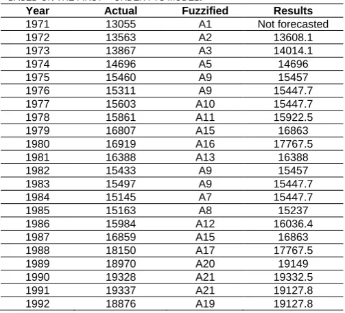
TABLE VI: FORECASTED ENROLMENTS OF UNIVERSITY OF ALABAMA
BASED ON THE FIRST – ORDER FTS MODEL.
Year Actual Fuzzified Results
1971 13055 A1 Not forecasted
1972 13563 A2 13608.1
1973 13867 A3 14014.1
1974 14696 A5 14696
1975 15460 A9 15457
1976 15311 A9 15447.7
1977 15603 A10 15447.7
1978 15861 A11 15922.5
1979 16807 A15 16863
1980 16919 A16 17767.5
1981 16388 A13 16388
1982 15433 A9 15457
1983 15497 A9 15447.7
1984 15145 A7 15447.7
1985 15163 A8 15237
1986 15984 A12 16036.4
1987 16859 A15 16863
1988 18150 A17 17767.5
1989 18970 A20 19149
1990 19328 A21 19332.5
1991 19337 A21 19127.8
1992 18876 A19 19127.8
To evaluate the forecasted performance of proposed method in the FTS, the mean square error (MSE) and the mean absolute percentage error (MAPE) are used as a comparison criterion to represent the forecasted
accuracy. The MSE value and MAPE value are computed according to (11) and (12) as follows:
MSE = 1
n∑ (Fi− Ri) 2 n
i=1 (4)
𝑀𝐴𝑃𝐸 = 1
𝑛∑ |
𝐹𝑖−𝑅𝑖 𝑅𝑖 | 𝑛
𝑖=1 ∗ 100% (5)
Where, Ri notes actual data on year i, Fi forecasted value on year i, n is number of the forecasted data
V. EXPERIMENTAL RESULTS
A. Experimental results for forecasting enrollments
In this subsection, we apply the proposed method for forecasting the enrolment of Alabama University from 1971s to 1992s are shown in Table 1.
Experimental results for our model will be compared with the existing methods, such as the SCI
model [2] the C96 model [3] and the H01 model [5] based on the first – order FTS are listed in Table 7 . Table 7 shows a comparison of MSE and MAPE of our method using the first-order fuzzy relation groups under different number of intervals, where MSE and MAPE are calculated according to (4) and (5) as follows:
𝑀𝑆𝐸 = ∑21𝑖=1(𝐹𝑖−𝑅𝑖)2
𝑁 =
(13608−13563)2+(14014.1−13867)2…+(19127−18876)2
21 = 56297
𝑀𝐴𝑃𝐸 = 1
21∑ |
𝐹𝑖−𝑅𝑖 𝑅𝑖 | 21
𝑖=1 ∗ 100% = 1 21(
𝑎𝑏𝑠(13608−13563)
13563 +
⋯ +𝑎𝑏𝑠(19127−18876)
18876 ) = 0.849%
where N denotes the number of forecasted data, Fi
denotes the forecasted value at time i and Ri denotes
the actual value at time i.
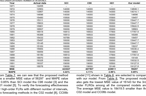
TABLE VII: A COMPARISON OF THE FORECASTED RESULTS OF PROPOSED MODEL WITH THE EXISTING MODELS BASED ON THE FIRST-ORDER FUZZY TIME
SERIES UNDER DIFFERENT NUMBER OF INTERVALS.
Year Actual data SCI C96 H01 Our model
1971 13055 - - - -
1972 13563 14000 14000 14000 13608.1
1973 13867 14000 14000 14000 14014.1
1974 14696 14000 14000 14000 14696
1975 15460 15500 15500 15500 15457
1976 15311 16000 16000 15500 15447.7
1977 15603 16000 16000 16000 15447.7
1978 15861 16000 16000 16000 15922.5
1979 16807 16000 16000 16000 16863
1980 16919 16813 16833 17500 17767.5
1981 16388 16813 16833 16000 16388
1982 15433 16789 16833 16000 15457
1983 15497 16000 16000 16000 15447.7
1984 15145 16000 16000 15500 15447.7
1985 15163 16000 16000 16000 15237
1986 15984 16000 16000 16000 16036.4
1987 16859 16000 16000 16000 16863
1988 18150 16813 16833 17500 17767.5
1989 18970 19000 19000 19000 19149
1990 19328 19000 19000 19000 19332.5
1991 19337 19000 19000 19500 19127.8
1992 18876 19000 19000 19149 19127.8
MSE 423027 407507 226611 56297
MAPE 3.22% 3.11% 2.66% 0.85%
From Table 7, we can see that the proposed method has a smaller MSE value of 56297 and MAPE value of 0.85% than SCI model the C96 model [3] and the H01 model [5]. To verify the forecasting effectiveness for high-order FLRs with different number of intervals
,
two forecasting methods in the C02 model [8], CC06bmodel [11] shown in Table 8, are selected to compare with our model. From Table 8, The proposed model also gets the lowest MSE value of 16143 for the 3rd-order FLRGs among all the compared models and The average MSE value is 18419.5 smaller than the C02 model and CC06b model.
TABLE VIII: A COMPARISON OF THE FORECASTED ACCURACY BETWEEN OUR MODEL AND C02 MODEL, THE CC06B MODEL FOR DIFFERENT INTERVALS
WITH DIFFERENT NUMBER OF ODERS BY THE MSE VALUE.
Methods Number of oders
2 3 4 5 6 7 8 9 Average(MSE)
C02 model 89093 86694 89376 94539 98215 104056 102179 102789 95868
CC06b model 67834 31123 32009 24948 26980 26969 22387 18734 31373
Our model 21300 16143 17040 18042 17837 17917 18931 20146 18419.5
To be clearly visualized, Fig. 1 depicts the trends for actual data and forecasted results of the H01 model with forecasted results of proposed method. From Fig. 1, It is obvious that the forecasting accuracy of the proposed model is more close than any existing models for the first-order fuzzy logical relationships with different number of intervals.
Vol. 2 Issue 10, October - 2016
Fig. 1: The curves of the H01 models and our model for forecasting enrolments of University of Alabama
Fig. 2: A comparison of the MSE values for different intervals with the high-order FTS model.
From Fig.2, it can see that the predicted values and the actual values are very close and the forecasting accuracy by the MSE value of the proposed model is more precise than among two compared models with different order fuzzy logical relationship.
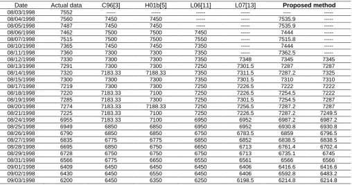
B. Experimental results for forecasting the TAIFEX
In this subsection, we present the forecasting results of the proposed model. Our model is validated
using the stock index data set of TAIFEX (Historical data of the TAIFEX in [11]). In order to verify the forecasting effectiveness of the proposed model with the high-order FLRGs and different numbers of intervals, six FTS models in C96 [3] model, H01b [5] model, L06[11] model, L07[13] model, are examined and compared. The forecasted accuracy of the proposed method is estimated using the MSE technique in equal (4).
TABLE IX: A COMPARISON OF THE FORECASTING VALUES OF THE PROPOSED MODEL BY MSE VALUE WITH EXISTING MODEL BASED ON 7TH –ORDER FTS
Date Actual data C96[3] H01b[5] L06[11] L07[13] Proposed method
08/03/1998 7552 --- --- --- --- ---- ---
08/04/1998 7560 7450 7450 --- --- 7535.9 ---
08/05/1998 7487 7450 7450 --- --- 7535.9 ---
08/06/1998 7462 7500 7500 7450 --- 7444 ---
08/07/1998 7515 7500 7500 7550 --- 7515.8 ---
08/10/1998 7365 7450 7450 7350 --- 7444 ---
08/11/1998 7360 7300 7300 7350 --- 7362.5 ---
08/12/1998 7330 7300 7300 7350 7348 7345 7345
08/13/1998 7291 7300 7300 7250 7301.5 7287 7287
08/14/1998 7320 7183.33 7188.33 7350 7311.5 7287.2 7325
08/15/1998 7300 7300 7300 7350 7301.5 7310 7310
08/17/1998 7219 7300 7300 7250 7226.5 7222 7222
08/18/1998 7220 7183.33 7100 7250 7226.5 7254.5 7222
08/19/1998 7285 7183.33 7300 7250 7301.5 7254.5 7287
08/20/1998 7274 7183.33 7188.33 7250 7256.5 7287.2 7287
08/21/1998 7225 7183.33 7100 7250 7226.5 7287.2 7249.5
08/24/1998 6955 7183.33 7100 6950 6952 6987.2 6987.2
08/25/1998 6949 6850 6850 6950 6952 6930.8 6930.8
08/26/1998 6790 6850 6850 6750 6783.5 6859 6796.5
08/27/1998 6835 6775 6775 6850 6852 6838.5 6838.5
08/28/1998 6695 6850 6750 6650 6713 6761.4 6702.4
08/29/1998 6728 6750 6750 6750 6713 6735.1 6745
08/31/1998 6566 6775 6650 6550 6561 6566 6566
09/01/1998 6409 6450 6450 6450 6406 6416.6 6416.6
09/02/1998 6430 6450 6550 6450 6406 6592.8 6483.2
09/03/1998 6200 6450 6350 6250 6198.5 6214.8 6214.8
1972 1974 1976 1978 1980 1982 1984 1986 1988 1990 1992 13,000
14,000 15,000 16,000 17,000 18,000 19,000 20,000
Years
N
um
be
r o
f st
ud
en
ts
Actual Data C96 model H01 model Our model
2 3 4 5 6 7 8 9
10,000 20,000 30,000 40,000 50,000 60,000 70,000 80,000 90,000 100,000 110,000
Order of FRLGs
M
SE
v
a
lu
e
09/04/1998 6403.2 6450 6450 6450 6406 6416.6 6416.6
09/05/1998 6697.5 6450 6550 6650 6703 6592.8 6702.4
09/07/1998 6722.3 6750 6750 6750 6713 6735.1 6725.2
09/08/1998 6859.4 6775 6850 6850 6852 6821.1 6861.5
09/09/1998 6769.6 6850 6750 6750 6783.5 6865.7 6768.3
09/10/1998 6709.75 6775 6650 6750 6713 6823.4 6716
09/11/1998 6726.5 6775 6775 6750 6713 6725.2 6725.2
09/14/1998 6774.55 6775 6775 6817 6783.5 6821.1 6780.8
09/15/1998 6762 6775 6775 6817 6783.5 6768.3 6768.3
09/16/1998 6952.75 6775 6850 6817 6953 6823.4 6930.8
09/17/1998 6906 6850 6850 6950 6952 6859 6930.8
09/18/1998 6842 6850 6850 6850 6852 6859 6847
09/19/1998 7039 6850 6850 7050 7089 7039 7039
09/21/1998 6861 6850 6850 6850 6852 6861.5 6861.5
09/22/1998 6926 6850 6850 6950 6952 6865.7 6930.8
09/23/1998 6852 6850 6850 6850 6852 6859 6861.5
09/24/1998 6890 6850 6850 6850 6893 6865.7 6898
09/25/1998 6871 6850 6850 6850 6852 6880.5 6880.5
09/28/1998 6840 6850 6750 6850 6852 6838.5 6838.5
09/29/1998 6806 6850 6850 6850 6792.5 6761.4 6820.5
09/30/1998 6787 6850 6750 6750 6783.5 6796.5 6796.5
MSE 9668.94 5437.58 1364.56 249.61 2538.43 187.18
From Table 9, we can see that the proposed method has the MSE value of 2538.43 smaller than the methods presented in C96 [3] and H01b [5] for the first-order fuzzy relationship groups with different number of intervals. Therefore, the proposed method obtains a lowest average MSE value of 187.18 among two forecasting models presented in L06 [11] and L07 [13] for the high-order fuzzy relationship groups with different number of intervals.
VI. CONCLUSIONS
In this paper, we have presented a hybrid forecasted method to handle forecasting enrolments of the University of Alabama and the TAIFEX based on the fuzzy logical relationship groups and automatic clustering algorithm. Firstly, the proposed method applies the automatic clustering algorithm to divide the historical data into clusters and adjust them into intervals with different lengths. Secondly, we fuzzify all the historical data of the enrolments and establish the fuzzy relation groups. Thirdly, we calculate forecasting output and compare forecasting accuracy with other existing models. Lastly, based on the performance comparison in Tables 7, 8 9 and Fig. 1, 2, it can show that our model outperforms previous forecasting models for the training phases with various orders and different interval lengths.
The proposed model was only tested by the forecasting enrollment problem and TAIFEX data, it can actually be applied to other practical problems such as earthquake forecast, and weather prediction in the further research.
ACKNOWLEDGMENT
The work reported in this paper has been supported by the Science Council of Thai Nguyen University of Technology - Thai Nguyen University, under contract number 110xHĐNCKH-ĐHKTCN
REFERENCES
[1] Q. Song, B.S. Chissom, “Forecasting Enrollments with Fuzzy Time Series – Part I,” Fuzzy set and system, vol. 54, pp. 1-9, 1993b.
[2] Q. Song, B.S. Chissom, “Forecasting Enrollments with Fuzzy Time Series – Part II,” Fuzzy set and system, vol. 62, pp. 1-8, 1994. [3] S.M. Chen, “Forecasting Enrollments based on Fuzzy Time Series,”
Fuzzy set and system, vol. 81, pp. 311-319. 1996.
[4] Hwang, J. R., Chen, S. M., & Lee, C. H. Handling forecasting problems using fuzzy time series. Fuzzy Sets and Systems, 100(1– 3), 217–228, 1998.
[5] Huarng, K. Heuristic models of fuzzy time series for forecasting. Fuzzy Sets and Systems, 123, 369–386, 2001b .
[6] Singh, S. R. A simple method of forecasting based on fuzzytime series. Applied Mathematics and Computation, 186, 330–339, 2007a.
[7] Singh, S. R. A robust method of forecasting based on fuzzy time series. Applied Mathematics and Computation, 188, 472–484, 2007b.
[8] S. M. Chen, “Forecasting enrollments based on high-order fuzzy time series”, Cybernetics and Systems: An International Journal, vol. 33, pp. 1-16, 2002.
[9] H.K.. Yu “Weighted fuzzy time series models for TAIEX forecasting ”, Physica A, 349 , pp. 609–624, 2005.
[10] Chen, S.-M., Chung, N.-Y. Forecasting enrollments of students by using fuzzy time series and genetic algorithms. International Journal of Information and Management Sciences 17, 1–17, 2006a. [11] Chen, S.M., Chung, N.Y. Forecasting enrollments using high-order
fuzzy time series and genetic algorithms. International of Intelligent Systems 21, 485–501, 2006b.
[12] Huarng, K. theH. Effective lengths of intervals to improve forecasting fuzzy time series. Fuzzy Sets and Systems, 123(3), 387–394, 2001a.
[13] Lee, L.-W., Wang, L.-H., & Chen, S.-M. Temperature prediction and TAIFEX forecasting based on fuzzy logical relationships and genetic algorithms. Expert Systems with Applications, 33, 539–550, 2007. [14] Jilani, T.A., Burney, S.M.A. A refined fuzzy time series model for
stock market forecasting. Physica A 387, 2857–2862. 2008. [15] Wang, N.-Y, & Chen, S.-M. Temperature prediction and TAIFEX
forecasting based on automatic clustering techniques and two-factors high-order fuzzy time series. Expert Systems with Applications, 36, 2143–2154, 2009
[16] Kuo, I. H., Horng, S.-J., Kao, T.-W., Lin, T.-L., Lee, C.-L., & Pan. An improved method for forecasting enrollments based on fuzzy time series and particle swarm optimization. Expert Systems with applications, 36, 6108–6117, 2009a.
[17] S.-M. Chen, K. Tanuwijaya, “ Fuzzy forecasting based on high-order fuzzy logical relationships and automatic clustering techniques”, Expert Systems with Applications 38 ,15425–15437, 2011.