On Inference of the Linear Regression Model with Groupwise Heteroscedasticity

(1)

with Groupwise Heteroscedasticity

Abdul Majid

Pakistan Bureau of Statistics, Pakistan [email protected]

Muhammad Aslam

Department of Statistics, Bahauddin Zakariya University, Pakistan [email protected]

Muhammad Amanullah

Saima Altaf

Abstract

The performance of heteroscedasticity consistent covariance matrix estimators (HCCMEs), namely, HC0, HC1, HC2, HC3 and HC4 have been evaluated by numerous researchers for the heteroscedastic linear regression models. This study focuses on examining the performance of these covariance estimators in case of groupwise heteroscedasticity. With the help of the Monte Carlo simulations, we evaluate the performance of these covariance estimators and the associated quasi-t tests. We consider the cases when data are divided into 10, 20 and 30 groups of different sizes and the regression is run on the mean values of the dependent variable and the regressor of these groups. The numerical results show that HCCMEs perform appealingly well in case of groupwise heteroscedasticity.

Keywords: Groupwise heteroscedasticity; HCCME; Size distortion; White’s estimator.

1. Introduction

The linear regression models for cross-sectional data often exhibit the problem of heteroscedasticity i.e. the error variances are not constant for all observations. In this situation, the ordinary least square (OLS) estimators of the parameters remain unbiased and consistent but become inefficient. Since the form of heteroscedasticity is usually unknown, the practitioners usually use the OLS estimators even when the error variances are not constant. However, the usual OLS covariance matrix estimator becomes biased and does not remain consistent when the homoscedasticity assumption is violated. Since the OLS standard errors are based directly on these variances, so the inferences drawn on the basis of these estimators become misleading and erroneous. It thus, becomes necessary to build and use alternative covariance matrix estimators that are consistent under both homoscedasticity and heteroscedasticity of unknown form. Several consistent covariance matrix estimators are available in the literature.

(2)

that they are valid in the presence of heteroscedasticity of unknown form. This is very convenient because it means we can report new statistics that work, regardless of the kind of heteroscedasticity present in the population”.

The most commonly used heteroscedasticity consistent covariance matrix estimator (HCCME) was presented by White (1980). White’s estimator is known as HC0 in the literature. MacKinnon and White (1985) and Davidson and MacKinnon (1993) presented three alternative improved versions of HCCMEs, commonly known as HC1, HC2 and HC3. Numerous researchers have evaluated the performance of HCCMEs for the heteroscedastic linear regression models (e.g., see Ahmed et al. 2011, Aslam et al. 2013, Cribari-Neto 2004, Cribari-Neto and Zarkos 1999, 2001, 2004, Flachaire 2005, Long and Ervin 2000, MacKinnon 2011 etc.).

In real life, there are many situations when the dependent and explanatory variables have to be aggregated as average values i.e. the means of dependent and explanatory variables are available and we have to run regression on these average values. As a result of such aggregation, the error tem in the resulting model becomes heteroscedastic, in spite of the fact that it is homoscedastic in the model of individual values. It is because the number of observations (say) n_g varies across the different groups. Such type of heteroscedasticity is called as groupwise heteroscedasticity (see Greene 2000, for more details). For groupwise heteroscedastic regression model, obviously, the usual OLS covariance matrix of estimates will be inconsistent. Thus, it becomes needful to use the HCCMEs. Now the question arises that what would be the performance of the HCCME in case of groupwise heteroscedasticity but the available literature is found to be silent in this situation. This thing motivated us to evaluate the performance of HCCMEs in case of groupwise heteroscedasticity. Using the Monte Carlo simulations, we evaluated the performance of HCCMEs for groupwise heteroscedasticity.

2. Heteroscedasticity-Consistent Covariance Matrix Estimator (HCCME)

Consider the regression model

yX  , (1)

where yis an n1 vector of observations on the dependent variable, X is an n p known design matrix of rank p,  is an p1vector of unknown parameters, and is an n1 vector of random errors with zero mean and variance 2 _,

n

I



  where In is an identity

matrix of order n.

The ordinary least squares (OLS) estimator is





1

ˆ

OLS X X X y

 _  _

 ,

and its covariance matrix is

 

ˆ





1





1

OLS

Cov   X X  XX X X  , (2)

where

 

.

(3)

If the errors are homoscedastic, then

 

2

.

E   I

So Eq. (2) becomes

 

ˆ ₂





1

.

OLS

Cov   X X 

Defining the residualse_i  y Xˆ_OLS, we can estimate the OLS covariance matrix (OLSCM) as

 

ˆ i2





1

OLS

e

OLSCM X X

n p

   





_, ₍₃₎

where n is the number of observations and p is the number of unknown parameters.

But if the errors are heteroscedastic and the form of heteroscedasticity is unknown then the HCCME, presented by White (1980), commonly known as HC0, can be used. White’s estimator is defined as





1

 

₂





1

0 _i .

HC  X X  X diag e X X X  

The disadvantage of White’s estimator is that it can be biased, usually downward, in small samples (see MacKinnon and White, 1985) and takes no account of the fact that OLS residuals tends to be too small. MacKinnon and White (1985) provided an improved estimator i.e., HC1, that was tailored after making the adjustment for the degree of freedom (d.f) as suggested by Hinkley (1977).





1 ₂





1

1 i

n

HC X X X diag e X X X

n p

 

    

 _{ }



= n HC0.

np

Another version of HCCME considered by MacKinnon and White (1985) is:





2





1 1

2 .

1

i

e

HC X X X diag X X X

h

   

  

 _ _

  

The ith squared OLS residual is weighted by the reciprocal of (1- h_i), where h_i is the ith diagonal element of the hat matrix, H X X X







1X.

The third HCCME is the jackknife estimator of Efron (1979, as modified by Davidson and MacKinnon, 1993) and is defined as:







2







1 1

2

3 .

1

i

e

h

   

  

  



 

 

(4)

versions of the HCCMEs in the linear regression model. Based on their simulation results, Long and Ervin showed that HC0 results in incorrect inferences when n ≤ 250

while other three versions of HCCMEs work well for small sample size, especially HC3. They strongly recommended that HC3 should be used for samples less than 250 regardless of the presence or absence of heteroscedasticity.

Cribari-Neto and Zarkos (2001) showed that HCCMEs do not perform well if there are high leverage points in the design matrix. They showed that the quasi-t tests based on HCCMEs mentioned above are not reliable in the presence of high leverage points in the design matrix. Cribari-Neto (2004) presented the HCCME that performs quite well in the presence of high leverage points in the design matrix. This estimator was named as HC4.













2

1 1

4 ,

1 i

i i e

h 

   

  

  



 

 

where

1

min 4, i min 4, i 4, i .

i n

i i

h nh nh

min

h p

h





 

  _ _

 

 

 _ _ _ _ _ _

  _ _  

 







The numerical results in Cribari-Neto (2004) showed that the asymptotic inferences in linear regression models were much affected by the presence of high leverage points in the design matrix. By the Monte Carlo simulations, Cribari-Neto (2004) showed that the quasi-t tests, based on the HC4 estimator, were reliable even in the presence of influential observations in the design matrix.

3. Groupwise Heteroscedasticity

The linear regression models are usually used in real life in which both the dependent and explanatory variables have individual values. There are many situations in real life, when the dependent and explanatory variable have aggregated or average values i.e. the means of dependent and explanatory variables are available and the regression is run for these average values. In spite of the fact that the error tem in the model of individual values is homoscedastic, when the observations are grouped and the regression is run on the means of dependent and explanatory variables, the error tem in the resulting model becomes heteroscedastic.

If the n observations are grouped into G groups each with n_g observations and the means

g

y and x_gfor g = 1, 2, …, G groups are observed then the regression model, given in Eq. (1), becomes

g g g

Y  X   (4)

or

.

g g g

(5)

The error term v_gin the above model is now heteroscedastic, irrespective of the fact that the error term in regression model (1) of individual values y_i and x_i, is homoscedastic because

 

2 2

( )

g Var vg Var g ng

     ,

where n_g is the number of observations in group G.

4. HCCME under Groupwise Heteroscedasticity

In case of groupwise heteroscedasticity, instead of the individual values, the mean of dependent variable is regressed on the means of explanatory variables. Consider regression model (4) where both, the dependent and independent, represent the respective mean values. For this model, White’s estimator can be written as

1 1

2

0 _i ,

HC X X X diag v X X X

 

  

  _{ }  

 _ _   _ _ (5)

where v_i  y X_OLS, are the OLS residuals for _OLS (X X )1X y .

After applying the degree of freedom adjustment, we get the HC1 estimator as

1 1

2

1 G _i ,

HC X X X diag v X X X

G p        _{ }    _ _ _{ } _ _     

= G HC0

Gp , (6)

where G is the number of groups which behaves like the sample size and p is the number of unknown parameters in groupwise heteroscedastic model.

The HC2 estimator can be written as

1 ₂ 1

2

1

i i v

r            _ _ _ _ _ _ 

  _ _   , (7)

where ri is the ith diagonal element of the hat matrix,

1

R X X X X



 

 

  

  .

The HC3 estimators becomes





1 2 1

2 3 . 1 i i v

r

   

  

   

_ _   _ _

  _  _   (8)

Finally, the HC4 estimator becomes





1 ₂ 1

4 ,

1 i

i i

v

r 

   

  

   

_ _   _ _

(6)

where

1

min 4, i min 4, i 4, i ,

i n

i i

r Gr Gr

min

r p

r





 

  _ _

 

 

 _ _ _ _ _ _

     

 







where r is the average of ri.

These estimators are used to get the consistent covariance matrix estimator of coefficient estimates for the model with groupwise heteroscedasticity.

5. Numerical Evaluation

The numerical results, presented in this study, were obtained using the simple regression model

i i

i x

y 0 1  ; i = 1, 2, …,n. (10)

We generated 275, 550 and 825 observations. For the case of 275 observations, the values of covariate x were obtained as random draws from the U (0, 1) distribution and then kept fixed. The errors_i’s were taken from the normal distribution with mean 0 and

variance 1 i.e. i~ N (0, 1). Clearly, the error term is homoscedastic with

2

i

 = 1. The dependent variable y was constructed using ₀ ₁ 1 under data generating process (DGP-I) and ₀ 10, ₁0.5 (DGP-II). These 275 observations were grouped into G = 10 groups each of size n_g where n_g = 5, 10, 15, …, 50 and the means y_gand x_g for all the 10 groups were obtained. It is obvious that 10

1

275

G

g j

n



 

 and that is why we, initially generated 275 observations. Then the simple regression was run on these average values as:

0 1

g g g

y   x  ; g = 1, 2, …, 10. (11)

The error term in the above model is now heteroscedastic irrespective of the fact that the error term in the regression model of individual values y_i and x_i is homoscedastic

because 2_g Var

 

_g 2 n_g where n_g is the number of observations in group G. Then these 275 observations were replicated twice and three times to get 550 and 825 observations, respectively. For such replication, the degree of heteroscedasticity remained unchanged to make comparisons for different data sets.

(7)

groups were observed. The regression for model (11) was run on the means of 20 and 30 groups, separately. These experiments were replicated 5000 times each for G =10, 20 and 30. The estimates of the ’s were computed by the OLS, and the estimates of

 

ˆ

OLS

Cov  were computed using Eq. (3) i.e. using the OLS and the HCCMEs, HC0,

HC1, HC2, HC3 and HC4, given in Eqs. (5)-(9), respectively. All the computations were performed through programming routines in the econometric package EViews 5.0 (visit www.eviews.com).

Following Cribari-Neto and Galvão (2003) and Cribari-Neto (2004), we computed the total relative bias (TRB) of the OLS, the HC0, HC1, HC2, HC3 and HC4 covariance estimators. The total relative bias yields the sum of the absolute relative biases of the estimated variances of ˆ0 and ˆ1. The relative bias is defined as the difference between

the mean value of variance estimator and the true value of variance divided by the true variance. Thus, the TRB is defined as

TRB =



 



 



 



 

0 0 1 1

0 1

ˆ ˆ ˆ ˆ

ˆ ˆ

.

ˆ ˆ

E Var Var E Var Var

Var Var

   

 

 



Table 1 and 2 presents the TRB under DGP-I and -II respectively for the OLS, HC0, HC1, HC2, HC3 and HC4 variance estimators.

Table 1: Total Relative Bias under DGP-I

G OLS HC0 HC1 HC2 HC3 HC4

10 0.78 1.41 1.27 0.56 2.96 70.39

20 0.74 0.72 0.58 0.13 0.83 4.31

30 0.79 0.81 0.72 0.50 0.10 0.95

Table 2: Total Relative Bias under DGP-II

10 1.15 2.91 2.47 1.12 3.31 38.32

20 1.23 1.19 0.97 0.44 1.83 3.51

30 1.29 1.22 1.13 0.97 1.21 1.79

(8)

HC3 and HC4 estimators reduces, dramatically but the similar behavior is not observed for the OLS, HC0, HC1 and HC2 estimators.

Again following Cribari-Neto (2004), we computed the root mean square error (RMSE) of the OLS, HC0, HC1, HC2, HC3 and HC4 estimators. Table 2 presents the square root of the total mean squared error ( 5000) for each variance estimator under consideration. It is defined as

 



ˆ ˆ0





ˆ

 

ˆ1



5000

RMSE MSE Var  MSE Var   ,

where

 







 





 



2

0 0 0

ˆ ˆ ˆ

MSE Var  Var Var   Bias Var  ,

and

 







 





 



2

1 1 1

ˆ ˆ ˆ

MSE Var  Var Var   Bias Var  ,

where Varˆ

 

ˆ₀ and Varˆ

 

ˆ₁ are the estimates of Var

 

ˆ₀ and Var

 

ˆ ,₁ respectively. The MSE thus comprises of not only bias but also the variance of different estimators.

Table 3: Total RMSE ( 5000) under DGP-I

10 63.01 83.47 79.21 93.76 387.63 6751.08

20 25.96 36.35 37.37 48.75 81.62 226.84

30 18.08 23.69 23.83 26.20 32.69 58.65

Table 4: Total RMSE ( 5000) under DGP-II

10 87.03 115.29 109.41 129.50 533.40 7324.62

20 34.86 50.21 49.61 66.33 112.73 213.37

30 23.97 32.72 32.91 36.19 45.15 81.01

Table 3 and 4 display the values of Total RMSE ( 5000) under DGP-I and –II, respectively for each variance estimator under consideration. The numerical results presented in Table 3 and 4 show that the OLS estimator yields the smallest RMSE as compared to other estimators under consideration for all G (number of groups). The HC4 estimator yields the largest RMSE as compared to other estimators. Cribari-Neto (2004) also reported the similar results but for the ungrouped data.

(9)

(in percentage) of quasi-t tests corresponding to the nominal level α = 1%, 5% and 10%, respectively. For convenience, we focus on the testing the null hypothesis 0

0: 1 1

H  

against the alternative hypothesisH₁: ₁ ₁0, where ₁0 is the true value of₁. The test statistic that has been used is

0

1 1

1

ˆ ˆ ˆ var( )

t  





 ,

where vaˆr(ˆ₁) denotes the estimate of variance of ˆ₁ obtained from the OLS and HCCMEs. Under the null hypothesis, the test statistic has a limiting normal distribution with zero mean and unit variance. The absolute values of test statistics thus obtained are compared with the critical values from this limiting distribution corresponding to the nominal level α = 1%, 5% and 10%.

Table 5: Estimated null rejection rates of quasi t-tests (α = 1 %) under DGP-I

10 8.34 24.50 20.22 13.14 6.10 1.94

20 6.10 10.26 9.00 7.26 5.10 2.46

30 14.02 18.94 17.56 15.52 12.64 9.22

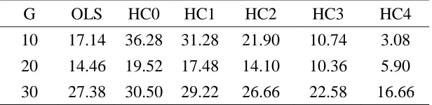
Table 5 presents the estimated NRR of the quasi t-tests corresponding to the nominal level α = 1% under DGP-I. The figures presented in Table 5 show that when G =10, the tests based on the HC0, HC1 and HC2 estimators result in larger size distortion. However, when G = 20, the performance of tests based on these estimators improves regarding size distortion. The tests that use the OLS, HC3 and HC4 estimators result in relatively less size distortion. We note that when G = 10 and 20, the tests based on the HC4 estimator, show satisfactory performance if the criterion is size distortion. For instance, when G = 10 and 20, the HC4-based test rejects the null hypothesis approximately 2% of the times that is close to the nominal level of the test. For G = 30, the tests based on all the covariance estimators, considered here, show large size distortion. However, the HC4 estimator results in less size distortion among rest of the estimators. Table 6 and 7 reveal the similar behavior for 5% and 10% level of significance, respectively under DGP-I. Table 8 presents the estimated NRR of the quasi

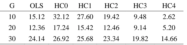
t-tests corresponding to the nominal level α = 5% under DGP-II. Almost similar behavior of NRR is observed under both DGP-I and DGP-II

Table 6: Estimated null rejection rates of quasi t-tests (α = 5 %) under DGP-I

10 17.14 36.28 31.28 21.90 10.74 3.08

20 14.46 19.52 17.48 14.10 10.36 5.90

(10)

Table 7: Estimated null rejection rates of quasi t-tests (α = 10 %) under DGP-I

10 24.92 43.62 38.78 28.92 14.68 4.38

20 22.22 27.08 24.86 20.34 15.06 9.10

30 35.48 38.58 37.08 34.24 30.08 23.18

Table 8: Estimated null rejection rates of quasi t-tests (α = 5 %) under DGP-II

10 15.12 32.12 27.60 19.42 9.48 2.62

20 12.36 17.24 15.42 12.46 9.14 5.20

30 24.14 26.92 25.68 23.34 19.82 14.66

Following Cribari-Neto and Lima (2009), we evaluated the performance of the OLS and HCCMEs, under groupwise heteroscedasticity, for interval estimation. The confidence intervals based on the OLS and HCCM estimators are constructed for 0 and 1. The

100(1-α) % two sided confidence intervals forj( j = 0, 1) are constructed as:

1 2

ˆ _{ˆ ( ),}ˆ

j Z  Var j

   

where ˆ_j are the OLS estimator of j and Varˆ ( )ˆj the is the estimator of

ˆ ( _j)

Var 

obtained by the OLS and HCCM estimators, under consideration. The nominal coverage of all the confidence intervals, under consideration, is 1  0.95. We compute the empirical coverage and average length of confidence intervals for the both coefficients

0

 and ₁ but for discussion here, we focus on ₁only.

Table 9 shows the empirical coverage and average length of confidence intervals for1,

(11)

Table 9: Confidence intervals for1: Coverage (%) and average length under DGP-I

Coverage Length Coverage Length Coverage Length Coverage Length Coverage Length Coverage Length

10 82.86 3.61 63.72 2.48 68.72 2.77 78.10 3.68 89.26 6.41 96.92 22.94

20 85.54 2.66 80.48 2.57 82.52 2.71 85.90 3.05 89.64 3.68 94.10 5.29

30 72.62 2.13 69.50 2.04 70.78 2.11 73.34 2.26 77.42 2.52 83.34 3.05

6. Conclusion

It is common practice to use the HCCMEs to get the consistent estimates of variances of the OLS estimates for heteroscedastic linear regression models. In many practical situations, averages of the dependent and explanatory variables are used and regression is run on these average values. In this situation, the problem of groupwise heteroscedasticity is evident. The present study unfolds the performance of the conventional HCCMEs to encounter groupwise heteroscedasticity by providing consistent covariance matrix estimates. Five versions of HCCME i.e. HC0-HC4, have been computed for the linear regression model, facing groupwise heteroscedasticity. The Monte Carlo results reveal that the HC3 and HC4 estimators perform adequately well in the presence of groupwise heteroscedasticity as they do in the usual heteroscedastic linear regression model. However, the HC4 estimator outperforms the HC3 estimator, giving less size distortion and better coverage in interval estimation.

References

1. Ahmed, M., Aslam, M. and Pasha, G. R. (2011). Inference under heteroscedasticity of unknown form using some adaptive estimator.

Communications in Statistics-Theory & Methods, 40, 4431-4457.

2. Aslam, M., Riaz, T. and Altaf, S. (2013). Efficient estimation and robust inference of linear regression models in the presence of heteroscedastic errors and high leverage points. Communications in Statistics- Simulation and Computation, 42, 2223-2238.

3. Cribari-Neto, F. (2004). Asymptotic inference under heteroskedasticity of unknown form. Computational Statistics & Data Analysis, 45, 215–233.

4. Cribari-Neto, F. and Galvão, N. M. S. (2003). A class of improved heteroskedasticity-consistent covariance matrix estimators. Communications in Statistics-Theory & Methods, 32, 1951–1980.

5. Cribari-Neto, F. and Lima, M. G. A. (2009). Heteroskedasticity-consistent interval estimators. Journal of Statistical Computation and Simulation, 79, 787-803.

(12)

7. Cribari-Neto, F. and Zarkos, S. G. (2001). Heteroskedasticity-consistent covariance matrix estimation: White’s estimator and the bootstrap. Journal of Statistical Computation and Simulation, 68, 391- 411.

8. Cribari-Neto, F. and Zarkos, S. G. (2004). Leverage-adjusted heteroskedastic bootstrap methods. Journal of Statistical Computation and Simulation, 74, 215- 232.

9. Davidson, R. and MacKinnon, J.G. (1993). Estimation and Inference in Econometrics. Oxford University Press, New York.

10. Efron, B. (1979). Bootstrap methods: Another look at the Jackknife. Annals of Statistics, 7, 1–26.

11. Flachaire, E. (2005). More efficient tests robust to heteroskedasticity of unknown form. Econometric Reviews, 24, 219-241.

12. Greene, W. H. (2000). Econometric Analysis. Prentice Hall, New Jersey.

13. Hinkley, D. V. (1977). Jackknifing in unbalanced situations. Technometrics, 19, 285–292.

14. Long, J. S., Ervin, L. H. (2000). Using heteroskedasticity consistent standard errors in the linear regression model. The American Statistician, 54, 217-224. 15. MacKinnon, J. G. (2011). Thirty years of heteroskedasticity-robust inference.

Queen’s Economics Department Working Paper No. 1268, Queen’s University, Canada.

16. MacKinnon, J. G. and White, H. (1985). Some heteroskedasticity consistent covariance matrix estimators with improved finite sample properties. Journal of Econometrics, 29, 305-25.

17. White, H. (1980). A heteroskedasticity-consistent covariance matrix estimator and a direct test for heteroskedasticity. Econometrica, 48, 817–838.