www.ijiset.com
Dealing Heteroscedasticity Problem in Regression Modeling
Using ML-Fisher Scoring Algorithm: Simulation Study
I Gede Nyoman Mindra Jaya
P 1*P
, Neneng Sunengsih
P 2P
1
P
Department Statistics, Padjadjaran University, Indonesia
P
2
P
Department Statistics, Padjadjaran University, Indonesia
*email: [email protected]
Abstract
The violation of the homoscedasticity assumption might lead to a misleading conclusion in regression modeling. When the variance error is a function of independent variables, the regression model may not be accurate, and the hypothesis testing might be invalid. We evaluated the maximum likelihood estimator using the fisher scoring approach, which is usually used to handle the heteroscedasticity problem in regression modeling. We also evaluate the performance of the ordinary least square estimator to see the serious effect of the heteroskedasticity problem on the accuracy, precision, and power of parameter estimation using the Monte Carlo simulation study. The maximum likelihood with the fisher scoring approach gives outperform estimates than the ordinary least square.
Keywords: Heteroscedasticity, Fisher Scoring, Ordinary least square, Maximum likelihood,
1. Introduction
Homoskedasticity is one of Gauss Markov's assumptions that usually hard to be fulfilled for the real data. This assumption assumes that the error term for each unit of the observation has a similar variance ( [1] [2] [3]). However, because of some conditions such as data collecting problem, outlier, omitted variable, and model specification may cause heteroscedasticity problem [2].
The violation of the homoscedasticity assumption because of some conditions which may lead to the inefficiency of the estimator. This assumption may not affect unbiased and consistent properties of maximum likelihood or ordinary least square estimators ( [2]). Although for some condition, the heteroscedasticity problem does not have consequences on unbiased properties, this condition can produce a wrong regression model. However, in the case of omitted variables, and those variables have a strong correlation with the error
term, the heteroscedasticity problem may lead to bias estimates and strongly influence the inference of the regression parameters. It might produce the misleading conclusion of the hypothesis testing. This condition shows that we have to pay attention to the violation of the homoscedasticity assumption to get the better model.
Many authors have considered variance modeling to have a correct standard error and confidence interval for mean in regression modeling [2]. There are several solutions have been proposed when the heteroscedasticity problem is related to the independent variables [1]. The variance error 𝜎𝑖2is modeled as (i) 𝜎𝑖2= (𝒛𝑖′𝜸), (ii)
𝜎𝑖2= (𝒛𝑖′𝜸)2, (iii) 𝜎𝑖2= (𝒛′𝑖𝜸)𝑝, (iv) 𝜎𝑖2= exp�(𝒛𝑖′𝜸)�. In case (iv), the log of the variance is a linear function of independent variables, which leads to a multiplicative heteroscedastic model [2]. There is the other way to model heteroscedasticity. However, this paper is focused on the model (i), (ii) and (iv).
In regression modeling, there is some estimator that usually used, such as ordinary least square (OLS), Maximum Likelihood, Bayesian method and machine learning ( [4] [5] [6] [7]). In this paper, we evaluate the biases and power tests of the first two methods to regression parameter inference.
The structure of the remainder of this paper is as follows. Section 2 presents the methodology. Section 3 applies simulation design. Section 4 presents the result and discussion, and section 5 presents the conclusions.
2. Methodology
2.1. Modeling heteroscedasticity problem
Assume we are modeling linear regression model with heteroscedasticity problem as below:
𝑦𝑖=𝐱𝑖′𝛃+ε𝑖; ε𝑖~𝑁(0,𝜎𝑖2),𝑖= 1, . . . ,𝑛 (1) where 𝑦𝑖 denotes the response variable for i-th unit observation, 𝐱𝑖= (𝐱𝑖1, … ,𝐱𝑖𝐾)′ denotes the K vector of
www.ijiset.com
(β0,β1, … ,β𝐾)′. The error term ε𝑖 is assumed follows normal distribution with un-constant variance. The variance 𝜎𝑖2 defined as 𝜎𝑖2=𝑔(𝒛𝑖,𝜸) with 𝒛𝑖=
(𝒛𝑖1, … ,𝒛𝑖𝐿) and 𝜸= (𝛾1, … ,𝛾𝐿)are the others covariates and its regression coefficients on the 𝜎𝑖2 with 𝑔(. ) is appropriate real function.
2.2. Ordinary least square (OLS)
OLS is the simple estimator that usually used to estimate regression parameters. The principal of OLS method is minimize the sum square error; 𝛃�= arg. min(∑ 𝜀𝑛𝑖 𝑖2). The OLS estimator is [8]:
𝛃�= (𝐱′𝐱)−𝟏𝐱′𝐲 (2)
OLS is the Best Linear Unbiased Estimator when all Gauss Markov assumption is satisfied. However, the violation of the homoskedasticity assumption leads to the inefficiency of parameter estimate and inconsistency of the standard error estimate. The inconsistency of the covariance matrix of the estimated regression coefficients, the tests of hypotheses, (t-test, F-test) are no longer valid. The weighted least square regression (WLS) to overcome the heteroscedasticity problem. However, defining the weight matrix becomes a new problem.
2.3. Maximum likelihood estimation using Fisher scoring algorithm
Maximum likelihood algorithm is a flexible algorithm to be used estimate the regression parameter when the heteroscedastic problem is found. The likelihood function is given by [9]:
𝐿(𝛃,𝜸|𝐲)≈ � �(𝜎1
𝑖2)1/2× 𝑛
𝑖=1
exp�− 1
2𝜎𝑖2(yi− 𝐱i ′𝛃)2��
(3)
and the log likelihood function can be written as:
ln𝐿(𝛃,𝜸|𝐲) =−12�ln
𝑛
𝑖=1
𝜎𝑖2
− 12�𝜎1
𝑖2(yi− 𝐱i ′𝛃)2 𝑛
𝑖=1
(4)
The parameter estimate of 𝛉= (𝛃,𝜸)′ are obtained by
𝛉�= argmax(ln𝐿(𝛃,𝜸|𝐲)) . However, there is no analytical solution for this function. Optimization method such as fisher scoring method can be used to obtain the parameter estimate of 𝛉.
The Fisher scoring method is based on the bloc diagonal Fisher information matrix to get maximum likelihood of the parameters interest [1]. An iterative algorithm of Fisher scoring method is given below [2]:
a) Given the initial value of 𝛃(𝟎) and 𝛄(𝟎)for the parameter. Usually we choose parameter estimate from OLS regression model.
b) 𝛃(𝒌+𝟏) is obtained from
𝛃(𝒌+𝟏)=�𝐱′𝑾(𝒌)𝐱�−𝟏𝐱′𝑾(𝒌)𝐲, where 𝑾(𝒌) =
diag�𝑤𝑖(𝑘)�,𝑤𝑖(𝑘)= 1/(𝜎𝑖2)(𝑘) and (𝜎𝑖2)(𝑘)=
exp�𝒛𝑖′𝜸(𝑘)�
c) 𝜸(𝑘+1) is obtained from
𝜸(𝑘+1)=�𝐳′𝑾(𝒌)𝐳�−𝟏𝐳′𝑾(𝒌)𝐲�, where 𝑾=1
2𝐈𝑛, with 𝐈𝑛 the 𝑛×𝑛 identity matrix, and 𝐲�is a 𝑛 -dimensional vector with i-th component:
y�𝑖=𝜂𝑖+𝜎1
𝑖2(yi− 𝐱i ′𝛃)2−1
(5) where 𝜂𝑖=𝑔(𝑧𝑖′𝜸)
d) Steps (b) and (c) will be repeated iteratively until the pre-specified stopping criterion is satisfied.
3. Simulation Design
We develop Monte Carlo simulation study to evaluate the bias and power of test of OLS, ML, and Bayesian approach in inferencing regression coefficient when the heterogeneity problem is found. There are two type heteroscedasticity functions were considered: 𝑔(𝑧𝑖′𝜸) =
(𝑧𝑖′𝜸)𝑝= (x1)𝑝;𝑝= {−2,−1,−0,1,2}. The systematic components for these models is defined follows Cordeiro (2008) [9].
𝜇=𝛽0+𝛽1x1 (6)
and for the variance
𝜎2=𝑥
1𝑝 (7)
www.ijiset.com
4. Result and Discussion
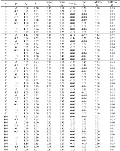
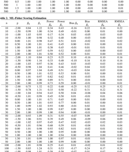
Table 1-2 give the sample means, power test, bias and mean square error of parameter estimate with ordinary least square and maximum likelihood estimator respectively for different number of sample (n) and power (p) of heteroscedasticity.
At first glance, it can be seen that for the estimated parameter has a negative bias or tends to underestimate while for the beta parameter estimate one has a positive bias or tends to overestimate.
Table 1. OLS Estimation
n p 𝛽0 𝛽1 Power
𝛽0
Power
𝛽1 Bias 𝛽0
Bias
𝛽1
RMSEA
𝛽0
RMSEA
𝛽1
www.ijiset.com
n p 𝛽0 𝛽1 Power
𝛽0
Power
𝛽1 Bias 𝛽0
Bias
𝛽1
RMSEA
𝛽0
RMSEA
𝛽1
300 -0.5 0.99 1.02 1.00 0.93 -0.01 0.02 0.01 0.02 300 0 1.00 0.99 1.00 1.00 0.00 -0.01 0.00 0.01 300 0.5 1.00 1.00 1.00 1.00 0.00 0.00 0.00 0.00 300 1 1.00 1.00 1.00 1.00 0.00 0.00 0.00 0.00 300 1.5 1.00 0.99 1.00 1.00 0.00 -0.01 0.00 0.01 300 2 1.00 1.00 1.00 1.00 0.00 0.00 0.00 0.00 500 -2 0.82 1.27 0.38 0.28 -0.18 0.27 0.18 0.27 500 -1.5 1.00 1.00 0.45 0.28 0.00 0.00 0.00 0.00 500 -1 0.99 1.02 0.91 0.67 -0.01 0.02 0.01 0.02 500 -0.5 1.00 1.00 1.00 0.99 0.00 0.00 0.00 0.00 500 0 1.00 1.00 1.00 1.00 0.00 0.00 0.00 0.00 500 0.5 1.00 1.00 1.00 1.00 0.00 0.00 0.00 0.00 500 1 1.00 1.00 1.00 1.00 0.00 0.00 0.00 0.00 500 1.5 1.00 1.00 1.00 1.00 0.00 -0.01 0.00 0.01 500 2 1.00 1.00 1.00 1.00 0.00 0.00 0.00 0.00
Table 2. ML-Fisher Scoring Estimation
n p 𝛽0 𝛽1 Power
𝛽0
Power
𝛽1 Bias 𝛽0
Bias
𝛽1
RMSEA
𝛽0
RMSEA
𝛽1
www.ijiset.com
n p 𝛽0 𝛽1 Power
𝛽0
Power
𝛽1 Bias 𝛽0
Bias
𝛽1
RMSEA
𝛽0
RMSEA
𝛽1
100 -0.50 0.99 1.02 0.84 0.77 -0.02 0.02 0.02 0.02 100 0.00 0.99 1.01 1.00 0.95 -0.01 0.01 0.01 0.01 100 0.50 1.00 1.00 1.00 1.00 0.00 -0.01 0.00 0.01 100 1.00 1.00 1.00 1.00 1.00 0.00 0.00 0.00 0.00 100 1.50 1.00 1.00 1.00 1.00 0.00 0.00 0.00 0.00 100 2.00 1.00 0.99 1.00 1.00 0.00 -0.01 0.00 0.01 300 -2.00 1.06 0.92 0.23 0.44 0.06 -0.08 0.06 0.08 300 -1.50 1.00 1.00 0.48 0.56 0.00 0.00 0.00 0.00 300 -1.00 0.99 1.01 0.91 0.83 -0.01 0.01 0.01 0.01 300 -0.50 0.99 1.02 1.00 0.99 -0.01 0.02 0.01 0.02 300 0.00 1.00 0.99 1.00 1.00 0.00 -0.01 0.00 0.01 300 0.50 1.00 1.00 1.00 1.00 0.00 0.00 0.00 0.00 300 1.00 1.00 1.00 1.00 1.00 0.00 0.00 0.00 0.00 300 1.50 1.00 0.99 1.00 1.00 0.00 -0.01 0.00 0.01 300 2.00 1.00 1.00 1.00 1.00 0.00 0.00 0.00 0.00 500 -2.00 0.88 1.17 0.23 0.43 -0.12 0.17 0.12 0.17 500 -1.50 1.00 0.99 0.30 0.58 0.00 -0.01 0.00 0.01 500 -1.00 0.99 1.02 0.95 0.89 -0.01 0.02 0.01 0.02 500 -0.50 1.00 1.00 1.00 1.00 0.00 0.00 0.00 0.00 500 0.00 1.00 1.00 1.00 1.00 0.00 0.00 0.00 0.00 500 0.50 1.00 1.00 1.00 1.00 0.00 0.00 0.00 0.00 500 1.00 1.00 1.00 1.00 1.00 0.00 0.00 0.00 0.00 500 1.50 1.00 1.00 1.00 1.00 0.00 0.00 0.00 0.00 500 2.00 1.00 1.00 1.00 1.00 0.00 0.00 0.00 0.00
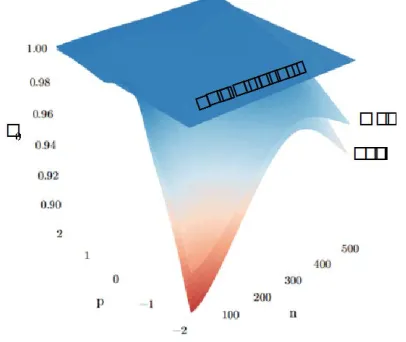
To provide a clear presentation of Table 1-2 we present the 3-D plot using smoothing loess function in Figure 1. Figure 1 present the detail information of the parameter estimate, bias, power test, and root mean square error for
different number of sample and power of heteroscedasticity
www.ijiset.com
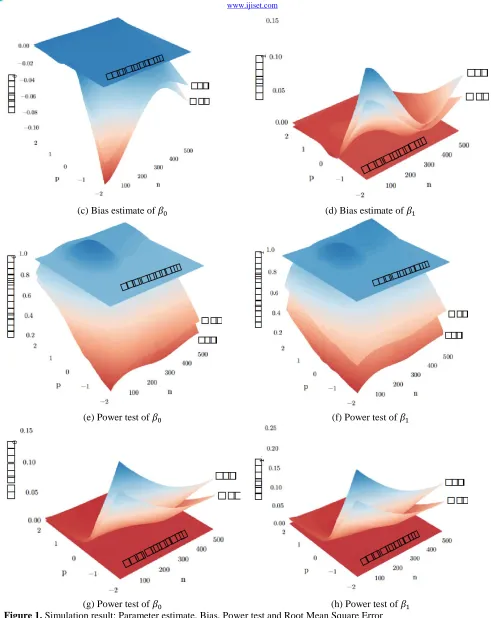
(c) Bias estimate of 𝛽0 (d) Bias estimate of 𝛽1
(e) Power test of 𝛽0 (f) Power test of 𝛽1
(g) Power test of 𝛽0 (h) Power test of 𝛽1
www.ijiset.com Figure 1 presents the detail of the comparison of ordinary
least square and maximum likelihood for heteroscedasticity problem using Fisher scoring approach. We present the parameters estimate, bias, power test, and root mean square error for different number of samples and different power of heteroscedasticity function.
We can see that the estimate of parameter intercept 𝛽0 tend to underestimate while for 𝛽1tend to overestimate.
For negative power (p), the effect of heteroscedasticity on parameters estimate, bias, power test, and root mean square error is getting worst even though the number of sample increases.
In general, the maximum likelihood with Fisher scoring method provides a better result compare that the ordinary least square.
IV. Conclusion
The violation of the homoscedasticity assumption might lead to a misleading conclusion in regression modeling. When the variance error is a function of independent variables, the regression model may not be accurate, and the hypothesis testing might be invalid. We evaluated ordinary least square which is not dealing with heteroscedasticity problem and maximum likelihood with fisher scoring which is dealing with heteroscedasticity problem. Monte Carlo simulation result shows that the the maximum likelihood with Fisher scoring method provides a better result compare that the ordinary least square. For negative power (p), the effect of heteroscedasticity on parameters estimate, bias, power test, and root mean square error is getting worst even though the number of sample increases.
Acknowledgments
The authors thank to the Rector Universitas Padjadjaran for facilitating this research.
Reference
[1] M. Aitkin, "Modelling Variance Heterogeneity in Normal Regression Using GLIM," Journal of the Royal Statistical Society, vol. 36, no. 3, pp. 332-339, 1987.
[2] E. Cepeda and D. Gamerman, "Bayesian Modeling of Variance Heterogeneity in Normal Regression Models," Brazilian Journal of Probability and Statistics, vol. 14, no. 2, pp. 207-221, 2000. [3] A. Sen and M. Srivastava, Regression Analysis
Theory, Methods, and Applications, New York: Springer, 1990.
[4] M. Blangiardo and M. Cameletti, Saptial and Spatio-Temporal Bayesian Model with R-INLA, John Wiley: United Kingdom, 2015.
[5] S. Geman and D. Geman, "Stochastic Relaxation, Gibbs Distributions, and the Bayesian Restoration of Images," IEEE Transactions on Pattern Analysis and Machine Intelligence, Vols. PAMI-6, no. 6, pp. 721-741, 1984.
[6] E. C. Cuervo and J. A. Achcar, "Regression Models with Heteroscedasticity using Bayesian Approach,"
Revista Colombiana de Estadística, vol. 32, no. 2, pp. 267-287, 2009.
[7] W. Wiedermann, R. Artner and A. v. Eye, "Heteroscedasticity as a Basis of Direction
Dependence in Reversible Linear Regression Models,"
Multivariate Behavioral Research, vol. 0, no. 0, pp. 1-20, 2017.
[8] G. Jude, Griffiths, C. Hill, H. Lutkepohl and T.-C. Lee, The Theory and Practice of Econometrics, Canada: 1985, John Wiley and Son.