Choosing Appropriate Regression Model in the Presence of Multicolinearity

(1)

ISSN Online: 2161-7198 ISSN Print: 2161-718X

DOI: 10.4236/ojs.2019.92012 Apr. 1, 2019 159 Open Journal of Statistics

Choosing Appropriate Regression Model in the

Presence of Multicolinearity

Maruf A. Raheem

1*

, Nse S. Udoh

2

, Aramide T. Gbolahan

3

1_{Department of Engineering and Mathematics, Sheffield Hallam University, Sheffield, UK} 2_{Department of Mathematics & Statistics, University of Uyo, Uyo,}_Nigeria

3_{Department of Computer Science, Sheffield Hallam University, Sheffield, UK}

Abstract

This work is geared towards detecting and solving the problem of multicoli-nearity in regression analysis. As such, Variance Inflation Factor (VIF) and the Condition Index (CI) were used as measures of such detection. Ridge Re-gression (RR) and the Principal Component ReRe-gression (PCR) were the two other approaches used in modeling apart from the conventional simple linear regression. For the purpose of comparing the two methods, simulated data were used. Our task is to ascertain the effectiveness of each of the methods based on their respective mean square errors. From the result, we found that Ridge Regression (RR) method is better than principal component regression when multicollinearity exists among the predictors.

Keywords

Multicollinearity, Adequacy, Regression coefficients, Variance Inflation Factor (VIF), Mean Square Error

1. Introduction

Regression Analysis is a statistical tool used in studying if there is existence of relationship, of any forms, either linear or nonlinear between the two variables, subject to certain constraints, such that one of the two variables can serve well to predict for the other. Meanwhile, it is important to note that our focus in this study is on the linear form of such relationship. Thus, when we talk of regres-sion, we only consider the linear regresregres-sion, which may either be simple, mul-tiple and or, multivariate in nature depending on the levels (or number) of va-riables on either side of the equation. When we compare a single dependent with a single independent variable, the regression is said to be simple, so we have How to cite this paper: Raheem, M.A.,

Udoh, N.S. and Gbolahan, A.T. (2019) Choosing Appropriate Regression Model in the Presence of Multicolinearity. Open Journal of Statistics, 9, 159-168.

https://doi.org/10.4236/ojs.2019.92012

Received: February 3, 2019 Accepted: March 29, 2019 Published: April 1, 2019

http://creativecommons.org/licenses/by/4.0/

(2)

DOI: 10.4236/ojs.2019.92012 160 Open Journal of Statistics simple (linear) regression. But, if only one dependent variable is being compared with more than one independent variables, the regression is said to be multiple in form; and thus we have multiple (linear) regression. The multivariate regres-sion (which is outside the scope of this research), only comes to play if we are comparing more than one level of the dependent variable with two or more le-vels of the independent variables.

1.1. Fundamental Principles

Consider the multiple regressions model:

0 1 1 2 2

i i i p pi i

Y =β +β X +β X + + β X +e (1)

In matrix form, (1) becomes:

Y =X′β + ∈ (2)

where in (1); βj s′ ∀ =j 1, 2,,p are the regression coefficients; Y n

(

×1

)

matrix

represents the outcome (response or dependent) variable and Xi s′ , ∀ =i 1, 2,,n are the explanatory (predictor or independent) variables, which are fixed and ei is the error term, which with Yi s′ are assumed to be random. With assumptions that: E e

( )

4) It may as well occur when in situations of nominal variables; the dummy variables are not properly use.

However, the following have been identified as the primary sources of multi-collinearity;

1) When a regression model is over defined; that is, including more than ne-cessary predictor variables in the model;

2) The data collection method is faulty; or better still choosing in appropriate sampling scheme used for data collection or generation;

3) Placing a spurious or unnecessary constraint on the model or in the popu-lation;

4) When the regression model is wrongly specified.

1.3. How Is Multicollinearity Detected?

There are a number of ways by which multicollinearity may be detected in a multiple regression model, which include:

1) when the correlation coefficients in the correlation matrix of predictor va-riables become so high that is close to one, or the value of correlation coefficient between two highly correlated predictor variables is close to one.

2) when the coefficient of determination (R2_{) value is so close to unity for a} particular predictor variable that is regressed on other independent variables to such an extent that the variance inflation factor (VIF) becomes so large [2].

3) When one or more eigenvalues of the correlation matrix becomes so small that is close to zero then multicollinearity is at work.

4) Another rule of thumb to detecting the presence of multicollinearity is that while one or more eigenvalues of the predictor variables become so small, to the extent of getting so close to zero but the corresponding condition number (ϕ) becomes very large [3] [4] [5].

5) Comparing the decisions made using overall F-test and t-test might provide some indication of the presence of multicollinearity. For instance, when the overall significance of the model is good using F-test, but individually, the coef-ficients are not significant using t-test, then the model might suffer from multi-collinearity

1.4. Possible Effects of Multicollinearity

(4)

DOI: 10.4236/ojs.2019.92012 162 Open Journal of Statistics 1) The partial contribution of each of the explanatory variable remains con-founded leading to difficulties in interpreting the model;

2) The variances as well as the coefficients of the predictor variables becomes un duly bogus (or inflated), thereby making precise estimation of the parameters becomes impossible;

3) The presence of multicollinearity gives rise to considerably high mean square error, paving ways for committing type-1-error;

4) The ordinary least square (OLS) estimators as well as their standard errors may be sensitive to small changes in the data, in order words, the results will not be robust; and

5) Finally, [6] observes that as multicollinearity increases, it complicates the interpretation of the variable because it becomes more difficult to ascertain the effect of any single variable, due to the variable interrelationships.

Since obtaining robust estimates of regression coefficients possess significant level of difficulties with ordinary least square (OLS) method, we in this research, we hope to explore other possible regression models; principal component re-gression (PCR) and ridge rere-gression (RR) methods as alternative techniques to estimating the model parameters, with a view to enhancing precision in esti-mating the parameters of the regression parameters when multicollinearity is suspected among the predictors without need for dropping any of the variables and that to determine which of the two methods perform better based on the mean square errors of the two models. Meanwhile, the use of condition number as well as variance inflation factor is endearing to us to check if multicollinearity exists among the covariates after estimating via OLS approach.

The remaining part of this paper is organized as follows; Section 2 has the brief discussion on the methodologies adopted while Section 3 presents the re-sults and general discussion on the findings of the research.

2. Methodology

This section discusses statistical techniques which are applied and compared with Ordinary Least Square (OLS) method in multiple linear regressions. These methods are Principal component regression (PCR) and Ridge regression (RR), their formulations as well as the underlining assumptions governing each of them are discussed.

2.1. Principal Component Regression (PCR)

(5)

com-DOI: 10.4236/ojs.2019.92012 163 Open Journal of Statistics ponents to effect a reduction in variance. The major goal of PCR include; varia-ble reduction, selection, classification as well as prediction. It would be recalled that this method is two procedural in application; first principal component analysis is applied, then the set of “k” uncorrelated or orthogonal component factors are used to replace the original p set of predictor variables. According to [7], PCR is a two-step procedure, in the first step, one computes principal com-ponents which are linear combinations of the explanatory variables while in the second step, the response variable is regressed on to the selected principal com-ponents. Combining both steps in a single method will maximize the relation to the response variables.

Let the random vector of the predictor variable be:

1, 2, 3, , p

X X X X

X′ =   _, with the covariance matrix Σ and eigenvalues

1 2 3 p 0

λ ≥λ ≥λ ≥≥λ ≥ . The linear combination:

i i

Y =e X′ ; (3)

Subject to the constraints:

( )

i i i; 1, 2, ,

Var Y =e e′Σ ∀ =i  p (4)

(

i, j

)

i j; , 1, ,2 , ;

Cov Y Y = Σe e′ ∀i j=  p i≠ j (5)

The principal components are those uncorrelated linear combinations

1, 2, 3, , P

Y Y Y Y whose variances are as maximal as possible.

Looking closely at the model (2), suppose X X′ = Σ is rewritten as P PΛ ′, with Λ_{being the}

(

p∗p

)

diagonal matrix of the eigenvalues of the design ma-trix or variance covariance mama-trix, Σ_and P= e e e₁, ₂, ,₃,ep representing associated normalized eigenvectors for the eigenvalues for Σ_{, such that:}

PP′=P P′ =I (Identity matrix) (6)

Rewriting the (2) by inserting (6) Z =XPP′β ε+ ; which then becomes:

Z= Φ +Y ε (7)

where Y =X P′ and Φ =P′β ; thus, Y Y′ =P X XP′ ′ = Σ =P P′ P P P P′ Λ ′ = Λ . The columns of Y, defined as the linearly uncorrelated components of the origi-nal random vector X are now the new set of orthogonal predictor variables; also known as the principal components. These now serve as the new covariates in the regression model, called principal component regression. Obtaining the es-timates of the model using OLS, we have:

1 1

ˆ _{Y Y Y Z}_′ − _′ −_{Y Z}_′

Φ = = Λ (8)

Such that the covariance of πˆ is

( )

2

( )

1 1 2

(

1 1 1

)

1 2

ˆ

k

V Φ =σ Y Y′ − = Λ−σ =diag λ− +λ− ++λ− (9)

(6)

DOI: 10.4236/ojs.2019.92012 164 Open Journal of Statistics gives much better result than the least square for prediction purpose.

2.2. Ridge Regression Method

This method was originally suggested by [9] as a procedure for investigating the sensitivity of least-squares estimates based on data exhibiting near-extreme mul-ticollinearity, where small perturbations in the data may produce large changes in the magnitude of the estimated coefficients.

The ridge regression estimate of the coefficients, βj; j=1, 2,,k are given

by

(

)

1

ˆ

R X X rI X Y

β _′ − _′

+

= (10)

where r≥0 is a constant called biasing factor, which needs to be set by the

re-searcher; such that when r = 0, the ridge regression automatically reduces to or-dinary least square. This is implies that ridge regression is an improved form of OLS, with minor transformation.

Thus:

( )

_ˆ

(

)

1

(

) (

1

) ( )

_ˆ

,

R R

E β = X X′ +rI − E X Y′ = X X′ +rI − X X E′ β =P β (11)

where

(

)

1

R

P = X X′ +rI − X X′ . This results point to the fact that ridge regression is a biased estimator of _βˆ_{, which is the necessary condition for getting away}

with the problem of estimating the model parameter.

Meanwhile the variance-covariance matrix of βR is obtained as:

( )

_ˆ

(

) (

1

)(

)

1 2

R

Var β = X X′ +rI − X X′ X X′ +rI − σ (12)

Giving rise to the mean square error:

( )

ˆ

R

MSE β =Bias+variance; i.e.

(

)

( )

2

ˆ ˆ

R R

Biasβ +Var β (13)

According to [10], ridge regressions are known to have favourable properties as shown by [9] βR has smaller mean square error than the ordinary least square estimators _βˆ_{, provided}σ2_{is small enough so that the validity of the}

regression model holds. [11] [12] also pointed out that the ridge regressions are known as shrinkage estimator.

3. Results and Discussion

In this work, we illustrate with an example to predicting gas productivity (Y) using density (X1), volumetric temperature (X2), sulphur content (X3), feedback flow (X4), output feedback temperature (X5), catalyst temperature in regenerator system (X6) and catalyst/feedback ratio (X7) as the independent variables.

(7)

[image:7.595.209.543.89.227.2]

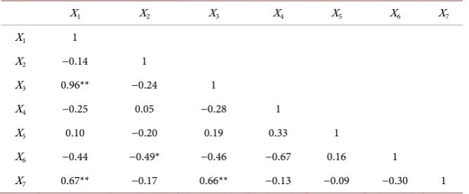
Table 1. Correlation matrix between independent variables.

X1 X2 X3 X4 X5 X6 X7

X1 1

X2 −0.14 1

X3 0.96** −0.24 1

X4 −0.25 0.05 −0.28 1

X5 0.10 −0.20 0.19 0.33 1

X6 −0.44 −0.49* −0.46 −0.67 0.16 1

X7 0.67** −0.17 0.66** −0.13 −0.09 −0.30 1

*P-value < 0.05, significantly correlated at 5%, **P-value < 0.01, significantly correlated at 1%.

significant possible relationships between X1 and X3 (r-0.96, P-value = 0.004), X3 and X7 (r = 0.66, P-value = 0.004). These results showed that there is presence of multicollinearity among these independent variables.

3.1. Multicollinearity Diagnostic

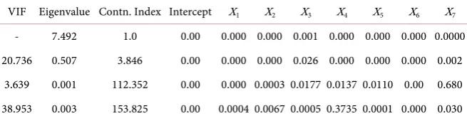
The existence of multicollinearity was investigated using Variance Inflation Factor (VIF), variables proportion and condition index. The result obtained is shown in Table 2. It could be confirmed that X1 and X3, have VIF greater than 10 which shows that there is collinearity problem.

Variance Inflation Factor (VIF)

The following VIF values were obtained from each of the Independent Va-riables:

( )

1 2 3

4 5 6

7

VIF 20.74, VIF 3.639, VIF 38.95,

VIF 2.58, VIF 2.82, VIF 5.58,

VIF 2.24

X X X

X

= = =

=

The result of VIF revealed presence of multicollinearity at VIF (1) and VIF (3) are greater than 10. This result confirmed a high level of multicollinearity among the independent variables.

The Condition Index (ϕ) = max min

λ

λ ; the ratio of maximum eigenvalue to

minimum eigenvalue.

7.492

749200

0.00001= . Since φ >1000 (749,200 > 1000), the results also

sup-ported that obtained from VIF. Mean Squared Error (MSE) For any given regression model:

SS

E E

MS

n p

=

− (14)

(8)

Table 2. Means square error for ordinary least, principal component and ridge regres-sion.

OLS PCR RR

0.70554 0.70553 0.68624

3.2. Summary of the Regresion Model

Ordinary Least Square (OLS)

GP 126.121 175.414 DTY 0.037 VT 2.121 SC 0.064 FF

0.042 FT 0.085 CT 1.718 FR

= − + − +

− + +

Principal Component Regression (PCR)

GP 51.400 2.336 DTY 0.336 VT 0.385 SC 0.552 FF

0.480 FT 0.674 Ct 0.049 FR

= − + − +

− + −

Ridge Regression (RR)

GP 54.1387 28.0014 DTY 0.0029 VT 0.5137 SC 0.0045 FF

0.0087 FT 0.1236 CT 0.62374 FR

= − + + +

+ + −

3.3. Comparison of OLS, PCR AND RR

Computing the mean Square Error for each of the model we obtain the following result. The result can be summarized in Table 2. From the table, it could be con-firmed that among the three estimates, ridge regression seems to produce the least mean square error; followed by the PCR and OLS. Though the difference between the MSE for PCR and OLS seems insignificant, this may be due to the data size used for the analysis.

Table 3 provides the results on the collinearity test obtained for the seven variables. In it we also have the VIF, Eigen-value and the conditional index.

4. Summary and Conclusion

Having fitted the respective regression models to the available data, we investi-gated the adequacies of the three models using the MSE square errors (see Table 2). It could be seen ridge regression gave the least error means square Error. Hence Ridge regression is considered superior.

Meanwhile, given the results obtained from the analyses, one may conclude there is no much difference in the error values, especially with the PCR and OLS; this may be due to the nature of the data used for the analysis. However, based on the results presented in Table 2, apparently the ridge regression performed better than principal components since it gave the smaller MSE value compared to PCR and OLS. The seeming insignificant difference between the MSE for PRC and OLS could be attributed to minimal level of multicollinearity between the covariates, except with X X1 7; X X1 3 and X X3 7 (see Table 1). The fact that

(9)

[image:9.595.210.538.90.175.2]

Table 3. Computations on collinearity test.

VIF Eigenvalue Contn. Index Intercept X1 X2 X3 X4 X5 X6 X7

- 7.492 1.0 0.00 0.000 0.000 0.001 0.000 0.000 0.000 0.0000 20.736 0.507 3.846 0.00 0.000 0.000 0.026 0.000 0.000 0.000 0.002

3.639 0.001 112.352 0.00 0.000 0.0003 0.0177 0.0137 0.0110 0.00 0.680 38.953 0.003 153.825 0.00 0.0004 0.0067 0.0005 0.3735 0.0001 0.000 0.030

Further, we observe that despite the little quantitative difference, there lie some advantages as well as disadvantages between the two methods. The advan-tages of RR method over PCR are that it is easier to compute and also provides a more stable way of moderating the model’s degrees of freedom than dropping variables [14]. Meanwhile, it is important to note that PCR affords us the op-portunity of testing a hypothesis to determine the most significant of the com-ponent variables.

Conflicts of Interest

The authors declare no conflicts of interest regarding the publication of this pa-per.

References

[1] Mansfiled, E.R. and Billy, P.H. (1982) Detecting Multicollinearity. The American Statisticians, 36, 158-160.https://doi.org/10.2307/2683167

[2] Hwang, J.T. and Netleton, D. (2000) Principal Component Regression with Data for Chosen Components and Related Methods. Technometrics, 45, 70-79.

https://doi.org/10.1198/004017002188618716

[3] Montgomery, D.C., Peck, E.A. and Vining, G.G. (2001) Introduction to Linear Re-gression Analysis. 3rd Edition, Willey, New York.

[4] Farrar, D.E. and Glanber, R.R. (1967) Multicollinearity in Regression Analysis. Re-view of Economic and Statistic, 49, 92-107.

[5] Myers, R.H. (1986) Classical and Modern Regression with Applications. 2nd Edi-tion, PWSKENT Publishing Company, USA.

[6] Hair, J.F., Anderson, R.E. and Black, W.C. (1998) Multivariate Data Analysis. 5th Edition, Prentice Hall, New Jersey.

[7] Filzmoser, P. and Groux, C. (2002) A Projection Algorithm for Regression with Collinearity. In: Jajuga, K., Sokołowski, A. and Bock, H.H., Eds., Classification, Clustering, and Data Analysis. Studies in Classification, Data Analysis, and Know-ledge Organization,Springer, Berlin, Heidelberg, 227-234.

[8] Martens, H. and Naes, T. (1989) Assessment, Validation and Choice of Calibration Method. In: Multivariate Calibration, 1st Edition, John Wiley & Sons, New York, 237-266.

[9] Hoerl, A.E. and Kennard, R.W. (1970). Ridge Regression: Biased Estimation for Non-Orthogonal Problems. Technometrics, 12, 55-67.

https://doi.org/10.1080/00401706.1970.10488634

(10)

DOI: 10.4236/ojs.2019.92012 168 Open Journal of Statistics Stockholm University, Stockholm.

[11] Marquardt, D.W. (1963) An Algorithm for Least-Squares Estimation of Nonlinear Parameters. Journal of Society of Industrial Applied Mathematics, 11, 431-441. [12] Marquardt, D.W. (1970) Generalized Inverses, Ridge Regression. Biased Linear

Es-timation, and Nonlinear Estimation, Techno Metrics, 12, 591-612. https://doi.org/10.2307/1267205

[13] Ijomah, M.A. and Nwakuya M.T. (2011) Ridge Regression Estimate. Unpublished M.Sc. Thesis, University of Port Harcourt, Port Harcourt.