www.nonlin-processes-geophys.net/19/291/2012/ doi:10.5194/npg-19-291-2012
© Author(s) 2012. CC Attribution 3.0 License.
Nonlinear Processes
in Geophysics
Grid preparation for magnetic and gravity data using fractal fields
M. Pilkington and P. Keating
Geological Survey of Canada, 615 Booth Street, Ottawa, ON, K1A 0E9, Canada
Correspondence to: M. Pilkington ([email protected])
Received: 20 January 2012 – Revised: 19 March 2012 – Accepted: 26 March 2012 – Published: 16 April 2012
Abstract. Most interpretive methods for potential field (magnetic and gravity) measurements require data in a grid-ded format. Many are also based on using fast Fourier trans-forms to improve their computational efficiency. As such, grids need to be full (no undefined values), rectangular and periodic. Since potential field surveys do not usually provide data sets in this form, grids must first be prepared to sat-isfy these three requirements before any interpretive method can be used. Here, we use a method for grid preparation based on a fractal model for predicting field values where necessary. Using fractal field values ensures that the statisti-cal and spectral character of the measured data is preserved, and that unwanted discontinuities at survey boundaries are minimized. The fractal method compares well with standard extrapolation methods using gridding and maximum entropy filtering. The procedure is demonstrated on a portion of a re-cently flown aeromagnetic survey over a volcanic terrane in southern British Columbia, Canada.
1 Introduction
Magnetic and gravity data are often subject to a number of processing or enhancement techniques designed to improve their interpretive value. These procedures, such as calcu-lating derivatives, downward continuation, reduction to the pole, can all be efficiently carried out in the frequency do-main using fast Fourier transforms (FFTs) (e.g., Kanasewich, 1981). FFT algorithms require that data exist at all points on the grid (i.e., there are no undefined values) and that the data are periodic with a period equal to the grid dimensions. Since magnetic and gravity data sets do not usually satisfy either of these requirements, they must be appropriately prepared be-fore FFT-based grid processing algorithms are used (Cordell and Grauch, 1982; Ricard and Blakely, 1988). FFT
algo-rithms can be based on powers of two or arbitrary factors. In the following we assume that a power of two FFT is used.
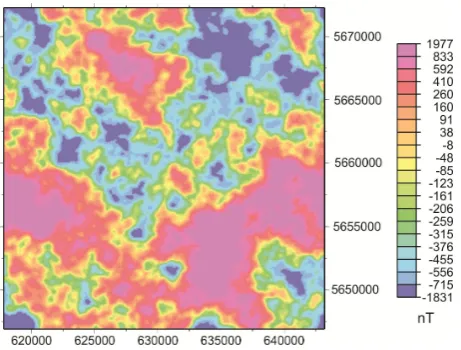
The shape of a survey is driven by a number of factors including the geology of the region being investigated, ac-quisition cost, flightline orientation and the configuration of the targeted geological feature, if known. As an example, Fig. 1 shows a portion of an aeromagnetic survey carried out in British Columbia. Standard gridding of this set of flight-line data produces a complex shaped grid (blue flight-line, Fig. 1) that must then be expanded to a rectangular form (black rect-angle, Fig. 1) so that there are no undefined values in the grid. The undefined parts of the grid must be populated by extrapolated values usually generated from the original grid-ded data. This expangrid-ded and now fully defined rectangular grid is, however, not yet in a form ready for applying FFT algorithms. The assumption of grid periodicity assumed in FFT algorithms must first be satisfied. In the simple case of a survey covering a rectangular area, one can remove the mean of the data, apply a tapering window to the data along the edges and pad the grid with zero values. The width of the tapering window should be about one tenth of the size of the grid. Use of a tapering window results in loss of data along the edges. Moreover, real surveys are seldom rectangular.
16
Fig. 1 Portion of the Bonaparte Lake aeromagnetic survey in British Columbia. Blue line is edge of gridded survey data. Black rectangle line is the outline of expanded rectangular grid. Coordinates in metres are UTM zone 21.
Fig. 1. Portion of the Bonaparte Lake aeromagnetic survey in British Columbia. Blue line is edge of gridded survey data. Black rectangle line is the outline of expanded rectangular grid. Coordi-nates in metres are UTM zone 21.
be tapered within a specified zone at the grid edges down to some average grid value, which then exists at all points around the grid perimeter. In practice the mean of the grid and in some cases a first-order trend should be removed be-fore processing. Linear trends are often present in data sets and cause large differences in values at opposite edges of the resulting grids; thus, the most expedient way to treat these ef-fects is to simply fit a low-order surface to the input grid and remove the trend. If necessary, this can be added back to the data after further processing. The width of the tapered zone must be large enough to smooth out any large magnitude dif-ferences between values at opposite grid edges. Padding or extrapolated regions at grid edges must have large widths, especially when three-dimensional (3-D) inversions of the data are done since fitting sources at depth will affect data at large horizontal distances. An alternative to tapering is to introduce extrapolated values that are already guaranteed to match and be periodic at the grid edges and do not contain large magnitude differences near to the grid perimeter. This is the technique used in the fractal approach below.
Where real and synthetic data meet (blue line, Fig. 1), extrapolated values need to fit seamlessly to the measured data and should preserve the statistical character of the input data as closely as possible. This ensures that discontinuities caused by a sudden change in wavelength and amplitude con-tent are avoided and that spurious wavelength components are not introduced into the extrapolated grid, which after fil-tering could affect values within the survey limits.
Common methods that are used for the extrapolation in-clude minimum curvature gridding (Briggs, 1974), mirror-ing the input data (Baranov, 1975, p. 42) and linear predic-tion filtering (Gibert and Galdeano, 1985). The two latter approaches are 1-D in that they act on the grid rows and
columns independently. Mirroring the data will preserve the frequency content of the original grid values, but when the input grid edges are irregular, the extrapolated values may require some smoothing to avoid large offsets between adjacent rows or columns in areas where extrapolated data are mirrored. Predicting data using maximum entropy pre-serves the original frequency content of the data along the columns and rows of the grid only up to how well the un-derlying autoregressive data model fits the observations. Op-erating on columns followed by rows or vice versa presents the same problems as the mirroring approach. Extrapolation using gridding has the advantage of being a 2-D approach. Nonetheless, the extrapolated values become much smoother than the input data as the distance from the survey grid edges increases. This smoothing changes the frequency content of the input data, which can have serious consequences on the final processed data grid.
The aim of this paper is to introduce an approach to grid preparation based on a fractal description of the data, whether gravitational or magnetic. The parameters of the fractal model are determined from the observed data and the synthesized fractal field used to extrapolate grid values into undefined regions where required.
2 Fractal description of potential fields
An alternative to existing approaches to grid preparation discussed in the previous section is to use knowledge of the character of the field so that any predicted values have the same statistical behaviour and frequency content as the known gridded values. Magnetic and gravitational fields have been shown to be well-described as fractal (Gregotski et al., 1991; Pilkington and Todoeschuck, 1993; 2004; Maus and Dimri, 1994; Lovejoy and Schertzer, 2007). Specifi-cally, the power spectrum of both fields is proportional to fβ, where f is the spatial frequency andβis the scaling expo-nent (the slope of the spectrum in log-log space). For gravity data, published values ofβ range from −4.5 to−5 based on regional and continent-wide data compilations (Maus and Dimri, 1996; Maus et al., 1998; Pilkington and Todoeschuck, 2004). Magnetic data show a wide range ofβ values be-tween−1 and−4.8, based on sample areas with scales from
studies is that a scaling or correlated type of description is more realistic than the earlier, commonly used assumption of an uncorrelated density/susceptibility distribution within the Earth’s crust.
Fedi et al. (1997) and Quarta et al. (2000) showed that magnetisation distributions other than a scaling one can also produce a scaling magnetic field power spectrum. Their models of uncorrelated distributions of blocks with constant magnetisation are spectrally equivalent to a scaling medium. A “blocky” distribution for magnetisation is not unrealistic since the basic approach of mapping magnetic units from magnetic field data involves assuming regions have similar susceptibilities and are associated with a single lithology. Nevertheless, susceptibility measurements from drill holes and rock sample suites over a wide range of scales support truly scaling properties of the underlying physical proper-ties. Furthermore, evidence of scaling behaviour has been provided through analyses using non-spectral methods. Sus-ceptibility logs were analysed with the rescaled range method and shown to be scaling by Leonardi and Kumpel (1996), while Dolan et al. (1998) demonstrated broad-band fractal scaling for several petrophysical logs based on four different calculation methods.
The fractal model of magnetic and gravity field data has already been exploited in a variety of uses including krig-ing of aeromagnetic data uskrig-ing a fractal covariance model (Pilkington et al., 1994), inversion for fractally magnetised source distributions (Maus and Dimri, 1995), Curie depth determination (Maus et al., 1997; Bouligand et al., 2009; Bansal et al., 2011), deriving accurate covariance models for satellite gravity data (Bansal and Dimri, 2005) and synthetic model-making to determine filtering parameters (Pilkington and Cowan, 2006). In the following, we outline a further use of fractals in the preparation of gravity and magnetic data grids prior to FFT-based processing and enhancement algo-rithms.
3 Method
Since we have a reliable model for predicting the character of crustal magnetic fields, we can use this knowledge to more realistically “fill in” and extrapolate grids before they are pro-cessed. The method we use is that of conditional simulation (Journel and Huijbregts, 1978; Tubman and Crane, 1995). This approach aims to produce synthesized values that have a specified statistical character and that match real values where known. For example, petroleum reservoir simulation to predict fluid flow requires a synthetic porosity distribution that matches those values measured in well-logs (Tubman and Crane, 1995). For the magnetic and gravity cases, the known values occur at all points within the survey area, but the important or conditioning data only occur at the survey edges, external or internal. The simulation approach needs to satisfy two requirements: one is that the simulated field has the same or very similar character to the measured field
17
Fig. 2. Spectra of the fractal grid upward continued to 125 m (continuous line) and the
measured magnetic data (dotted line).
Fig. 2. Spectra of the fractal grid upward continued to 125 m (con-tinuous line) and the measured magnetic data (dotted line).
and the other is that the simulated values match those at the original survey grid boundaries.
To create a synthetic fractal field, we generate Gaussian white noise (which has a flat power spectrum) with a spec-ified mean (M) and standard deviation (σ). These values are Fourier transformed and multiplied by fβ/2 whereβ is the required scaling exponent (Pilkington et al., 1994). To account for the distance between the top of the source dis-tribution (usually assumed to be ground level) and the mea-surement altitude, the synthetic field values are upward con-tinued in the frequency domain. The grid is also projected to the same geomagnetic latitude as the observed data (Blakely, 1996). Finally, inverse Fourier transformation gives the de-sired field. This synthetic grid is then scaled to the same standard deviation as the measured grid.
4 Data example
18
Fig. 3. Synthetic fractal magnetic grid upward continued to a height of 125 m. Note the periodicity of the grid. Top and bottom edges are identical as well as left and right edges. Coordinates in metres are UTM zone 21.
Fig. 3. Synthetic fractal magnetic grid upward continued to a height of 125 m. Note the periodicity of the grid. Top and bottom edges are identical as well as left and right edges. Coordinates in metres are UTM zone 21.
area. The major northwest-southeast trending positive mag-netic anomaly is interpreted to be caused by Nicola volcanics buried beneath thin (<25 m), Chilcotin Group cover. Else-where in the region, Nicola Group volcanics are commonly associated with high-amplitude (commonly >1000 nT and rarely >4000 nT) anomalies. Regions with Kamloops or Chilcotin volcanic rocks generally exhibit a spotty magnetic fabric, lacking any dominant coherent trends.
Figure 2 shows the power spectrum of the field in Fig. 1. A fractal field with similar character to the measured field was then determined based on the observed power spectrum. The parameterβcan be estimated from the slope of the long wavelength part of the measured spectrum. This slope will be modified slightly when the fractal field is upward continued to the average terrain clearance (125 m). Matching the power level is easily done once a trial spectrum is plotted. A scaling parameterβ= −2.5 was estimated from the observed data spectrum and used for the generated fractal field shown in Fig. 3. This grid has a 256×256 cell dimension and is the size of the final extrapolated grid. How much to extend the measured data will be constrained by the shape of the orig-inal grid, but should be large enough to allow for a smooth transition from original data out to the edge of the extended grid. In our experience, an extrapolation zone of width equal to 10 % of the original grid dimensions appears to be suffi-cient (cf., Fig. 1). The power spectrum of the synthetic data grid (Fig. 3) is shown in Fig. 2, where a good match with the observed spectrum is apparent. The observed spectrum shows a fall-off in power at the longest wavelengths (>20 km) compared to the synthetic values. This difference is of-ten seen and is interpreted to be caused by the limited depth extent of magnetic sources (Maus et al., 1997; Bouligand et al., 2009).
19
Fig. 4. Synthetic fractal grid extrapolated to rectangular edges after removal of fractal data located outside the survey area outline in blue in Fig. 1. Edges are zeros. Coordinates in metres are UTM zone 21.
Fig. 4. Synthetic fractal grid extrapolated to rectangular edges after removal of fractal data located outside the survey area outline in blue in Fig. 1. Edges are zeros. Coordinates in metres are UTM zone 21.
20
Fig. 5. Conditioned field given by the field in Fig. 4 subtracted from the field in Fig. 3. This conditioned grid is zero at the observed field grid edges (blue line, Fig. 1) and within the survey area. Coordinates in metres are UTM zone 21.
Fig. 5. Conditioned field given by the field in Fig. 4 subtracted from the field in Fig. 3. This conditioned grid is zero at the observed field grid edges (blue line, Fig. 1) and within the survey area. Coordi-nates in metres are UTM zone 21.
21
Fig. 6. Magnetic data after extrapolation to a rectangular area. Measured data remain unchanged. Edges are zero. Coordinates in metres are UTM zone 21.
Fig. 6. Magnetic data after extrapolation to a rectangular area. Mea-sured data remain unchanged. Edges are zero. Coordinates in me-tres are UTM zone 21.
5 Conclusions
Fractal extrapolation is an alternative to commonly used grid extrapolation techniques. In these techniques, periodicity is obtained by padding the grid with zeros after extrapolation, based on maximum entropy prediction or extrapolation of the grid using minimum curvature or inverse distance gridding. In the case of non-rectangular grids with irregular edges, this can lead to complex algorithms. Mirroring rectangular grids is rather simple, but can be very complex for irregu-larly shaped grids. The proposed technique is obtained from a series of simple steps that are easy to implement. The tech-nique is independent of the shape of the survey. As seen in the real data example, the extrapolated grid does not show
22
Fig. 7. Final grid after fractal extrapolation. The grid is now periodic. Coordinates in metres are UTM zone 21.
Fig. 7. Final grid after fractal extrapolation. The grid is now peri-odic. Coordinates in metres are UTM zone 21.
23
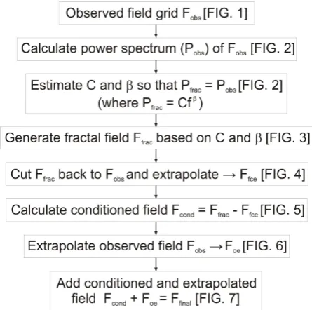
Fig. 8. Flow chart summarizing the steps required for fractal grid extrapolation. Where quantities have been plotted, the appropriate figure number is indicated. The expressions used for different quantities (e.g., Fobs) are not used in the text but used here for brevity. Fig. 8. Flow chart summarizing the steps required for fractal grid extrapolation. Where quantities have been plotted, the appropriate figure number is indicated. The expressions used for different quan-tities (e.g., Fobs)are not used in the text but used here for brevity.
any discontinuities along the edges of the survey; for other extrapolation techniques this can only be obtained by signif-icant programming effort. The main advantage of the fractal method is that the extrapolated grid has the same frequency content as the original grid.
Edited by: L. Aliouane
Reviewed by: A. Biswas and another anonymous referee
References
Bansal, A. R. and Dimri, V. P.: Self-affine gravity covariance model for the Bay of Bengal, Geophys. J. Int., 161, 21–30, 2005. Bansal, A. R., Gabriel, G., Dimri, V. P., and Krawczyk, C. M.:
Esti-mation of depth to the bottom of magnetic sources by a modified centroid method for fractal distribution of sources: An applica-tion to aeromagnetic data in Germany, Geophysics, 76, 11–22, 2011.
Baranov, W.: Potential fields and their transformations in applied geophysics, Gebruder Borntraeger, Berlin, 121 pp., 1975. Blakely, R. J.: Potential Theory in Gravity and Magnetic
Applica-tions, Cambridge University Press, 441 pp., 1996.
Bouligand, C., Glen, J. M. G., and Blakely, R. J.: Mapping Curie temperature in the western United States with a fractal model for crustal magnetization, J. Geophys. Res., 114, B11104, doi:10.1029/2009JB006494, 2009.
Briggs, I. C.: Machine contouring using minimum curvature, Geo-physics, 39, 39–48, 1974.
Cordell, L. and Grauch, V. J. S.: Reconciliation of the discrete and integral Fourier transforms, Geophysics, 47, 237–243, 1982. Dolan, S., Bean, C., and Riollet, B.: The broad-band fractal
na-ture of heterogeneity in the upper crust from petrophysical logs, Geophys. J. Int., 132, 489–507, 1998.
Fedi, M.: Global and local multiscale analysis of magnetic suscep-tibility data, Pure Appl. Geophys., 160, 2399–2417, 2003. Fedi, M., Quarta, T., and de Santis, A.: Inherent power-law
behav-ior of magnetic field power spectra from a Spector and Grant ensemble, Geophysics, 62, 1143–1150, 1997.
Gettings, M. E.: Multifractal magnetic susceptibility distribution models of hydrothermally altered rocks in the Needle Creek Igneous Center of the Absaroka Mountains, Wyoming, Non-lin. Processes Geophys., 12, 587–601, doi:10.5194/npg-12-587-2005, 2005.
Gibert, D. and Galdeano, A.: A computer program to perform transformations of gravimetric and aeromagnetic surveys, Comp. Geosci., 11, 5, 553–588, 1985.
Gregotski, M. E., Jensen, O. G., and Arkani-Hamed, J.: Frac-tal stochastic modeling of aeromagnetic data, Geophysics, 56, 1706–1715, 1991.
Journel, A. G. and Huijbregts, C. J.: Mining Statistics, Academic Press, New York, 600 pp., 1978.
Kanasewich, E. R.: Time sequence analysis in geophysics, Univ. of Alberta Press, Edmonton, Alberta, 480 pp., 1981.
Leonardi, S. and Kuempel, H. J.: Scaling behaviour of vertical magnetic susceptibility and its fractal characterization; an exam-ple from the German Continental Deep Drilling Project (KTB), Geol. Rundsch., 85, 50–57, 1996.
Lovejoy, S., Pecknold, S., and Schertzer, D.: Stratified multifractal magnetization and surface geomagnetic fields–I, Spectral analy-sis and modelling, Geophys. J. Int., 145, 112–126, 2001. Lovejoy, S. and Schertzer, D.: Scaling and multifractal fields in
the solid earth and topography, Nonlin. Processes Geophys., 14, 465–502, doi:10.5194/npg-14-465-2007, 2007.
Maus, S. and Dimri, V.: Fractal properties of potential fields caused by fractal sources, Geophys. Res. Lett., 21, 891–894, 1994. Maus, S. and Dimri, V.: Potential field power spectrum inversion
for scaling geology, J. Geophys. Res., 100, 12605–12616, 1995. Maus, S. and Dimri, V.: Depth estimation from the scaling power spectrum of potential fields?, Geophys. J. Int., 124, 113–120, 1996.
Maus, S., Gordon, D., and Fairhead, J. D.: Curie-depth estimation using a self-similar magnetization model, Geophys. J. Int., 129, 163–168, 1997.
Maus, S., Fairhead, J. D., and Green, C. M.: Improved ocean geoid resolution from retracked ERS-1 satellite altimeter waveforms, Geophys. J. Int., 134, 243–253, 1998.
Pilkington, M. and Todoeschuck, J. P.: Fractal magnetization of continental crust, Geophys. Res. Lett., 20, 627–630, 1993. Pilkington, M., Gregotski, M. E., and Todoeschuck, J. P.: Using
fractal crustal magnetization models in magnetic interpretation, Geophys. Prosp., 42, 677–692, 1994.
Pilkington, M. and Todoeschuck, J. P.: Scaling nature of crustal susceptibilities, Geophys. Res. Lett., 22, 779–782, 1995. Pilkington, M. and Todoeschuck, J. P.: Power-law scaling behaviour
of crustal density and gravity, Geophys. Res. Lett., 31, L09606, doi:10.1029/2004GL019883, 2004.
Pilkington, M. and Cowan, D. R.: Model-based separation filtering of magnetic data: Geophysics, 71, L17–L23, 2006.
Quarta, T., Fedi, M., and de Santis, A.: Source ambiguity from an estimation of the scaling exponent of potential field power spectra, Geophys. J. Int., 140, 311–323, 2000.
Ricard, Y. and Blakely, R. J.: A method to minimize edge effects in two-dimensional discrete Fourier transforms, Geophysics, 53, 1113–1117, 1988.
Thomas, M. D. and Pilkington, M.: New high-resolution aeromag-netic data: A new perspective on geology of the Bonaparte Lake map area, British Columbia, Geological Survey of Canada, Open File 5743, 3 Sheets, 2008.