R E S E A R C H P A P E R
Open Access
Accurate laser scanner to camera
calibration with application to range sensor
evaluation
Peter Fuersattel
1,2*, Claus Plank
3, Andreas Maier
1and Christian Riess
1Abstract
Multi-modal sensory data plays an important role in many computer vision and robotics tasks. One popular
multi-modal pair is cameras and laser scanners. To overlay and jointly use the data from both modalities, it is necessary to calibrate the sensors, i.e., to obtain the spatial relation between the sensors.
Computing such a calibration is challenging as both sensors provide quite different data: cameras yield color or brightness information, laser scanners yield 3-D points. However, several laser scanners additionally provide reflectances, which turn out to make calibration to a camera well feasible. To this end, we first estimate a rough alignment of the coordinate systems of both modalities. Then, we use the laser scanner reflectances to compute a virtual image of the scene. Stereo calibration on the virtual image and the camera image are then used to compute a refined, high-accuracy calibration.
It is encouraging that the accuracies in our experiments are comparable to camera-camera stereo setups and outperform another of other target-based calibration approach. This shows that the proposed algorithm reliably integrates the point cloud with the intensity image. As an example application, we use the calibration results to obtain ground-truth distance images for range cameras. Furthermore, we utilize this data to investigate the accuracy of the Microsoft Kinect V2 time-of-flight and the Intel RealSense R200 structured light camera.
Keywords: Laser scanner, Range camera, RealSense R200, Kinect V2
1 Introduction
Finding the spatial relation between a laser scanner and a 2-D or 2.5-D camera is crucial for sensor data fusion. Knowing this relation enables a multitude of applications, for example coloring the point cloud, the generation of textured meshes, or the creation of high accuracy ground truth for range cameras. The method proposed in this work has been specifically designed for generating refer-ence distances for range camera evaluation. Nonetheless, the approach is not limited to this application and can also be used to calibrate a common 2-D camera to a laser scanner.
Range cameras find widespread use, for example in the field of robotics [1], in space [2, 3], automation in
*Correspondence: [email protected]
1Pattern Recognition Lab, University of Erlangen - Nuremberg, Martensstrasse
3, Erlangen, Germany
2Metrilus GmbH, Henkestrasse 91, Erlangen, Germany
Full list of author information is available at the end of the article
logistics [4] or in augmented reality devices like the Google Tango phones. The major problem with these sen-sors is their limited accuracy. This gives rise to thorough camera evaluations with respect to accuracy and other individual camera characteristics that influence the range measurements.
Several studies that investigate the accuracies and error characteristics of range cameras have been presented in the past. Rauscher et al. [5] analyze range cameras with respect to their applicability to robotics. Yang et al. pre-sented a detailed study on the Kinect V2 [6]. Fuersattel et al. evaluated multiple time-of-flight cameras with respect to different error sources [7]. Wasenmüller and Stricker compare the structured light Kinect V1 camera to the time-of-flight-based Kinect V2 camera [8].
Quantitative evaluation of range cameras requires scenes with ground truth distance measurements. Nair et al. state three methods to acquire such ground truth [9]:
• Computed from a calibration pattern and known camera intrinsic parameters
• Computed from a calibration pattern as seen from a second high-resolution camera with known intrinsic parameters and known spatial relation to the evaluated camera.
• Measured with an additional, highly accurate 3-D sensor (e.g., a laser scanner) with known spatial relation to the evaluated camera.
The first two approaches have limited information value as they typically provide reference distances only for pla-nar regions. Moreover, the accuracy of the ground truth quickly degrades as the distance between camera and calibration pattern increases.
A laser scanner mitigates both issues. Laser scan-ners typically provide high-accuracy point clouds of a scene for larger operating ranges than camera-based solu-tions. Also, this distance information can be obtained for arbitrary, not necessarily planar, surfaces. However, to leverage laser scanner point clouds for range camera evaluation, it is necessary to calibrate the laser scanner to the camera.
In this paper we propose a method for solving this task. Starting from a scene that shows multiple calibration pat-terns, e.g., checkerboards, we show how stereo calibration methods can be used to obtain the rotation and transla-tion between the sensors. We aim at calculating the spatial relation based on a single point cloud/camera image pair, as acquiring densely sampled point clouds can take up to multiple minutes.
First, a virtual image of the point cloud has to be gen-erated. It is important that this image shows all calibra-tion patterns without occlusions. Thus, we demonstrate how the laser scanner’s unordered point cloud can be transformed such that it is approximately aligned with the coordinate system of the camera. From this trans-formed point cloud, a virtual image is generated. In this image, the pixel intensities are derived from the reflectiv-ity data that is associated with the individual 3-D point measurements.
The reflectivity data quantifies the amount of light that is reflected from a point in the scene back to the laser scanner. Therefore, the strong contrast of the calibration patterns also results in strong variations of the reflectiv-ity data. By detecting the calibration patterns in both the virtual and the camera image, point correspondences for the two sensors can be obtained with sub-pixel accuracy. Finally, these corresponding points are used as input to established stereo calibration algorithms to obtain the spatial relation between both sensors. Note that it is necessary that the scene is sampled densely, such that at least one 3-D point measurement can be mapped to each pixel of the virtual image. Dense point clouds are required
for example calculating accurate meshes of the scene, or like in our application, for generating ground-truth distance measurements for range cameras. In this work, we exploit the high sampling density to achieve even more accurate calibration results than current state-of-the-art methods.
The proposed method is evaluated with multiple data sets from four different range cameras. We show both qualitatively and quantitatively that the presented method aligns the coordinate systems accurately and, further-more, considerably outperforms the baseline method. In image domain, misalignments of less than 0.2 pixels are achieved. For corresponding 3-D coordinates in the scene, the mean error is as small as 1.3 mm.
The contributions of this work consist of two parts.
1. We present an automatic method for calibrating a laser scanner to a camera. This method enables the user to estimate the spatial relation between the two sensors with a single shot of a scene, which contains only a small number of calibration patterns. The applicability of the proposed method is shown for four different camera-laser scanner setups.
2. We use the calibration technique to present accuracy evaluations for different range camera technologies: the Microsoft Kinect V2 time of flight camera and Intel RealSense R200 structured light cameras.
In Section 2 we present related work. Detailed informa-tion on the proposed algorithm can be found in Secinforma-tion 3. The evaluation of the performance of the presented approach and the range camera evaluation results are pre-sented in Section 4. Section 5 summarizes and concludes this work.
2 Related work
Several approaches exist for calibration of laser scanners to cameras. Oftentimes, these methods are categorized by the type of laser scanner they operate on, namely methods for line scanners and methods for 2.5-D laser scanners.
plane-line correspondences to constrain the estimation. This method also requires fewer plane-line pairs than the method by Zhang et al. [10].
Line laser scanners obtain range information only for a single scanline. In the context of range camera evaluation, this information is not sufficient. Instead, dense 2.5-D point clouds are preferable. For example, Unnikirshnan et al. [13] published an interactive Mat-lab toolbox to calculate the spatial relation between a camera and a 2.5-D dense point cloud. The authors rec-ommend using at least 15 to 20 images. In each of the images, the calibration pattern region has to be delim-ited manually by drawing a polygon that encloses the area. In contrast, we find the planar segments of the calibration pattern automatically. With multiple patterns in the scene, an accurate calibration from a single shot is possible. The method proposed by Geiger et al. [14] obtains the spatial relation based on a single shot of a scene that shows mul-tiple checkerboard patterns. Based on the checkerboards and planar segments in the scene, an initialization for a subsequent iterative closest point-based refinement is cal-culated. In contrast to their work, we incorporate the laser scanner amplitudes to reduce the impact of inaccuracies of the plane detection.
Ha et al. [15] propose a new, specifically constructed calibration pattern with a triangular hole to reduce the number of calibration images. While other methods typ-ically require at least three different poses of calibra-tion patterns, this method requires only two. Hoang et al. [16] also use a calibration pattern with a triangu-lar hole. Their pattern is used to obtain 3-D/2-D corre-spondences for solving the perspective-n-point problem. Gong et al. [17] propose to use as a calibration tar-get three planes that form a trihedral. Based on at least two shots on such scenes, the relative transformation between the two sensor coordinate systems is estimated via nonlinear optimization. Although the method does not require special calibration targets, it still requires the user to define the planar region in the camera image. Our method requires three patterns, but these are off-the-shelf patterns without particular manufacturing requirements.
Moghadam et al. [18] estimate the spatial relation from line segments that can be detected both in the point cloud and in the camera image. Taylor and Nieto [19] find the spatial relation by maximizing the mutual infor-mation between the camera image and a virtual image, which is colored according to the direction of the point cloud’s normals. The work presented in [20] extends this method by a more robust normal estimation algorithm. However, both methods share the same drawbacks: the usage of particle swarm optimization requires (a) the initial knowledge of the range of the extrinsic param-eters and (b) a computationally expensive rendering
of a virtual image for each particle in each iteration. In contrast, we propose to use scene reflectivity to gener-ate virtual views, which enables the use of highly accurgener-ate calibration targets. Pandey et al. [21] also do not require a calibration target. The authors propose a calibration via minimizing the mutual information between the cam-era pixels and the laser scanner reflectivity information. This approach requires multiple views in order to obtain a smooth cost function that can be optimized robustly. Levinson and Thrun proposed a framework that mon-itors the accuracy of a calibrated camera-laser scan-ner setup while being in use [22]. If a miss-calibration is observed, the extrinsic parameters are corrected by finding the transformation which maximizes the over-lap between edges in the image and in the point cloud. This approach requires multiple frames and varied scene geometry such that sufficient corresponding edges can be found and a smooth cost function can be obtained. Scott et al. [23] presented an approach for the calibration of a laser scanner and cameras setup that also exploits reflec-tivity information. The method is suited for setups that move through an environment, e.g., in an autonomous driving scenario. The authors relax the constraint that field of views at a single point in time must overlap. Instead, the authors assume that some overlap will occur at some later point in time due to motion of the rigid sensor setup. The abovementioned methods are partic-ularly useful if no calibration pattern is present, e.g., outside a lab environment. However, the disadvantage of these approaches is the reduced accuracy compared to controlled lab setups.
3 Laser scanner to camera calibration
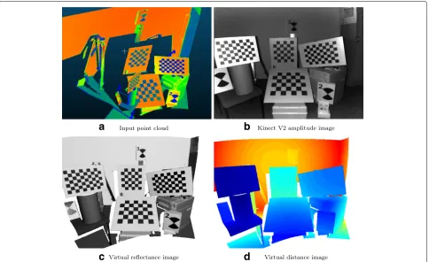
a
b
c
d
Fig. 1Examples from a Kinect V2 / laser scanner setup.aLaser scanner data, visualized in a point cloud viewer.bAmplitude image of the Kinect V2 for reference.c,dVirtual reflectance and distance images of the point cloud as seen from the camera position
much more difficult or even cause complete failure. We mitigate this problem by computing a virtual image that shows the calibration patterns from an angle similar to the observing camera. It is likely that there is consid-erable overlap between such computed virtual image and the camera image. Thus, we seek a transformation that approximately aligns the camera and laser scanner coordinate systems.
In the next subsections, we present the full calibration algorithm in three steps, i.e.,
1. Finding the plane segments of the calibration patterns in the unordered point cloud 2. Calculation of an initial alignment for the two
coordinate systems
3. Virtual image generation and estimation of a spatial relation via stereo calibration
3.1 Finding the calibration patterns in the point cloud We assume that planes within certain size boundaries stem from calibration patterns. We first search such planes in the unordered point cloud obtained from the laser scanner. The algorithm uses the idea that a plane is characterized by a set of co-located points with surface
normals pointing towards the same direction. We define neighborhoods for individual points and normal-based region growing.
In organized point clouds, the term neighborhood is often defined as the 4-connected or 8-connected neigh-borhood of a(x,y) coordinate of a 2-D array. This asso-ciation is not available with unorganized point clouds. In this work, we define the neighborhood of a pointpias its
No closest points in aL2 sense. These neighbors can be efficiently looked up by organizing the point cloud in a suitable data structure, for example an Octree. The nor-malnifor a pointpican be approximated by fitting a plane to the point and itsNo neighbors. This can be done effi-ciently by calculating the eigenvalue decomposition of the covariance matrix of these points [24].
pi= ⎛ ⎝pi+
No
j=0
wijpj ⎞
⎠ ⎛⎝1+ No
j=0
wij ⎞
⎠ , (1)
wherewij=e
αpi−pj2
e(βni−nj1) , (2)
andpjdenotes thejth neighbor ofpi. The same smooth-ing can also be applied to each normalni. The influence of the distance between points and the difference between normals is controlled with the parametersαandβ.
The computed normals are used to segment planar seg-ments in the point cloud. The algorithm begins with a random seed point to define a new planar segment. The seed point consists of a point coordinate and its associ-ated normal. We perform breadth-first region growing on points with similar normals. In other words, all points in the neighborhood of the segment that have a similar nor-mal are iteratively added to the current segment. Every time a new point has been added to a segment, its nor-mal is updated to be the average nornor-mal of all supporting points. The similarity of two normals is determined by thresholding on their angular difference. In our experi-ments, a conservative threshold of 10° has proven to work well. Segmentation stops if all points have been assigned to a segment label. The segmentation is similar to a pre-vious method for approximate plane segmentation for organized point clouds [25].
With all points assigned to a planar segment, we select those segments that may represent calibration patterns. Assuming that the dimensions of the calibration patterns are known, it suffices to threshold on the sizes of the minimum oriented bounding boxes of all segments.
3.2 Estimation of the initial spatial relation
The initial transformation approximately aligns the coor-dinate system of the laser scanner and the camera. The initialization is calculated from the candidate planes and the planes derived from the checkerboard patterns visible in the camera image.
First, the checkerboard patterns have to be detected as accurately as possible in the camera image. In this work we use the detector proposed in [26]. With the known dimensions of the patterns and the intrinsic parameters of the camera, the 3-D coordinates of the calibration features (e.g., checkerboard corners) can be calculated. Correspon-dences between planes in the laser scanner and detected patterns in the camera image can be directly established if the calibration patterns can be uniquely identified by their size, and if the number of plane candidates matches the number of calibration patterns. Otherwise, these cor-respondences have to be estimated. The naive solution is to evaluate all possible permutationsK for planes and patterns and to choose the permutation that minimizes some error metric. IfNccalibration patterns are used, then
Ncplane candidates are drawn from all found plane can-didates. The centroids of the plane segments m(p) and the calibration patternsm(c)are used as candidate corre-spondences to estimate a transformationR. The optimum transformationR∗is the one that minimizes the following error metric
R∗
i =argmin K
Nc
i
Rm(ic) −m(ip). (3)
The quality of a permutation is measured as the sum of the distances between the transformed centroids Rm(ic) and the centroids of the respective planar seg-mentsm(ip). Under the assumption that calibration pat-terns and planes have been accurately detected, then the minimum of the error metric corresponds to the best ini-tialization. Note that other metrics could be employed here as well, e.g., metrics based on normal directions or combinations of normal directions and centroids. How-ever, we found the metric in Eq. (3) to be sufficient, since the initialization requires only a rough estimate of the spatial relation. In our experiments, the number of per-mutationsKto search through was always low, since most plane candidates are already filtered out using the sizes of the calibration patterns.
The calculation above imposes mild constraints on the positions and orientations of the calibration patterns. These constraints are identical to the requirements for a robust stereo calibration and typically not difficult to sat-isfy: to obtain the most accurate results, the checkerboard poses must constrain all six degrees of freedom of the rigid body transformation. In practice, this means that the checkerboards need to point into different directions (see, e.g., Fig. 1b) and should cover as much area of the field of view as possible.
3.3 Virtual view generation and refinement transformation via stereo calibration
The initial, approximate alignment of the point cloud with the camera image can be used to perform stereo calibra-tion. To this end, a virtual image is computed from the point cloud. Virtual image and camera image together are then used to obtain a second transformation that refines the initial relation between the sensors.
Brightness differences in the virtual image are cre-ated from reflectivity information at each point from the laser scanner. Strong reflectivity variations within the cal-ibration pattern result in strong contrasts in the virtual image. This is particularly useful at the transition between black and white quads of the checkerboard pattern for calibration.
have to be defined such that the calibration patterns can be detected reliably. In this work, (p) will be used to denote the projection from a point pin 3-D space onto a point (u,v) image plane, with containing the pin-hole camera parameters as well as potential lens distortion parameters.
If the camera itself has a reasonable resolution, then their intrinsic parameters can also be used for the virtual camera. Otherwise, these parameters need to be selected manually. It is possible to distinguish two cases: first, if the camera resolution is very low, for example with time-of-flight cameras, then a higher image resolution should be chosen. In contrast, if the image resolution of the camera is very high (e.g.,> 1280×1024), the point cloud might not be dense enough to provide good amplitude values for each pixel. In the latter case, the resolution needs to be adjusted to a smaller value.
The simplest method to obtain the intensity informa-tion for each pixel is to project all points of the point cloud onto the image plane. First, the intensities C(p) of all points which are projected onto a single pixel coordinate (u,v) have to be obtained. To this end, we define a function γ (u,v,p), which indicates whether a point p is projected onto a particular (u,v) coordinate or not.
γ (u,v,p)= ⎧ ⎨ ⎩
true if(p)→(u,v),
|u−u| ≤0.5∧ |v−v| ≤0.5 false otherwise
LetN =
pj|γ (u,v,pj)
be the set of all points that are projected on pixel(u,v). As a simple heuristic to mitigate issues from occlusions, we limit the size ofN to a maxi-mum of 8. If more than 8 points map onto(u,v), we select only the 8 points that are closest to the camera. Then, the intensityV(u,v)of the virtual image is given as the average ofNclaser scanner intensity valuesC(pj),
V(u,v)= 1 Nc
pj∈N
C(pj). (4)
Instead of the naive approach, more sophisticated methods can be used to obtain intensity values, for example ray casting. However, this is beyond the scope of this work.
Next, the calibration patterns are detected in the vir-tual image and matched to the keypoints from the camera image. These correspondences can be used to compute a second rigid body transformation R∗r, which we call refinement transformation. R∗r is obtained by minimiz-ing the reprojection error between correspondminimiz-ing key-points as given in Eq. (6). The cost function measures the
2-D distance between a keypointxiand its corresponding transformed and projected keypointxˆiin the other image.
R∗r =argmin Rr
i
xi−Rrˆ−1(xˆi)
(5)
+xˆi− ˆRr−1−1(xi)
, (6)
whereˆ denotes the projection from the point cloud to the virtual image. The inverse projections−1andˆ−1 are obtained by solving the perspective-n-point prob-lem. Note that there are also direct solutions to calculate rotations and translations for 3-D point correspondences, for example the method by Horn [27]. By choosing the nonlinear optimization approach, we can jointly optimize both forR∗r and the transformation which relates the cal-ibration pattern coordinate system and the camera coor-dinate system, thereby achieving a more accurate refine-ment transformation. By concatenating R∗i and R∗r, the final spatial transformationRf is obtained. Knowing the final rigid body transformation, it is possible to directly transform any point cloud into the coordinate system of the camera. This transformed point cloud allows the cal-culation of virtual amplitude images or virtual distance images that are accurately aligned with the camera image.
4 Evaluation
A particular benefit of a laser scanner-to-camera calibra-tion is the ability to create ground truth for evaluating range sensors. To this end, we use two classes of range sen-sors as cameras: time-of-flight (ToF) sensen-sors (Microsoft Kinect V2 and PMD CamBoard Pico Flexx) and structured light sensors (Intel RealSense R200 and the Orbbec Astra). The laser scanner is a Leica ScanStation P20 scanner.
In case of the ToF cameras, the amplitude channel is used to capture the calibration scene. For calibrating the structured light cameras to the laser scanner, we use the infrared channels with the pattern emitter either being covered or disabled. Of the RealSense R200’s two infrared channels, we choose the left one as it is aligned with the distance map.
Whenever possible, we used the factory calibration of the range cameras as provided by the individual camera SDKs. For all cameras, except the Astra, these parame-ters could be obtained. The latter was calibrated with 60 checkerboard images using the method by Zhang [28].
the initial alignment. In order to create common basis for comparison, we replace the proposed stereo calibration-based refinement with the ICP-calibration-based refinement. To this end, we generate 3-D coordinates from the camera intrin-sics and the checkerboard coordinates as suggested by the authors.
The setup of our experiments and the used data is described in Section 4.1. In Section 4.2, we present qual-itative results for the proposed method. In Section 4.3, we present quantitative results on the evaluation scenes. Section 4.4 provides additional insights on the impact of the proposed refinement step. An evaluation of the mea-surement accuracy of a ToF (Kinect V2) and a structured light camera (RealSense R200) conclude the evaluation in Section 4.5.
4.1 Experimental setup and data
We captured five different scenes with the same spatial relation: a calibration scene that shows the four patterns, an evaluation scene with rearranged patterns, and three general scenes with different objects. The individual point clouds contain ≈ 6.2 million points, sampled from a volume of approximately 230×150×95 cm.
In the calibration and evaluation scene, four checker-board patterns with different dimensions and a different number of corners are captured:
• 6×5inner corners, 66.67 mm corner spacing • 6×7inner corners, 50 mm corner spacing • 6×9inner corners, 44 mm corner spacing • 8×7inner corners, 50 mm corner spacing
All patterns are printed on rigid boards to avoid errors from bending calibration patterns. Captured images are averaged for 100 frames to reduce the impact of measure-ment noise. The spatial relation between the laser scanner and the cameras is calculated on the first scene.
In all amplitude, intensity, and virtual images shown in the evaluation, the pixel values are normalized to values between 0 and 1 for better comparison.
4.2 Qualitative evaluation results
We illustrate the performance of the proposed method by comparing virtual reflectance images with observed images. The calibrations between the individual cameras and the point cloud are calculated on the first scene. Then, calibration data is used to generate virtual images of the evaluation scene for each camera. For comparison, each camera has been calibrated with the proposed method and the baseline method to the point cloud.
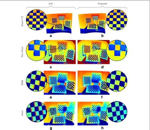
Figure 2 shows the difference between the observed camera images and the virtual images for the baseline method (denoted as “ICP”) and for the proposed method (denoted as “Proposed”). Wrong spatial relations show
as additional edges in the scene, whereas all edges in the scene coincide for an accurate transformation. It is important to emphasize that the magnitude of the pixel differences is not caused by misalignments, but by the internal conversion of the incoming light to intensities of the different sensors.
When calculating the spatial parameters with the base-line method, small offsets between corresponding edges can be observed (see Fig. 2a, e, and g). In contrast, for the proposed method, the virtual and observed images accu-rately coincide for all cameras. A visual comparison of the calibration results of the CamBoard Pico Flexx is difficult due to the low sensor resolution and the low reflectance of the black checkerboard patches. In these areas, the Cam-Board Pico Flexx does not provide amplitude values, as only a small portion of the emitted light is reflected back to the sensor.
4.3 Quantitative results
The reprojection error is a common choice to eval-uate the quality of a stereo calibration result. Thus, we compare the checkerboard positions in the cam-era image and in the virtual image. In this experiment, the system is calibrated on the first scene. Hereafter, the reprojection errors are calculated on the evaluation scene. As the virtual image is generated from the per-spective of the camera, we can directly compare the 2-D positions of the keypoints which are returned by the checkerboard detection algorithm.
For assessing the impact of the misalignments in 3-D, we reproject the keypoints based on the intrinsic param-eters and known pattern dimensions. Similarly, as in the 2-D case, we can directly compute the differences between corresponding 3-D world coordinates.
The results of this comparison are shown in Table 1. With the proposed method, we observe mean errors in corresponding 3-D coordinates between ≈ 1 to 3 mm, depending on the used camera. When relying only on 3-D information, like in the ICP variant, the measured errors are at least three times as large as for the proposed approach.
The calibration errors of the proposed method are within the expectation of typical stereo calibrations. The authors of the pattern detector report 3-D measurement errors between 1 and 7 mm, depending on the sensor resolution [26].
4.4 Influence of the refinement transformation
Fig. 2Difference of observed image and the corresponding virtual images for the two evaluated approaches. The difference images (a), (c), (e) and (g) have been calculated with virtual images generated with calibrations from the ICP-based approach. The figures (b), (d), (f) and (h) show overlays which have been calculated with calibrations from the proposed method. For the baseline method, misalignments can be observed in examples (a), (e) and (f). In contrast, no misalignments identified if the proposed method is used for calibration
initial transformation has only limited accuracy. The cen-troid is given by the mean coordinate of all points that belong to the segment, and thus sensitive to segmentation errors. If the segmentation for example contains points of the supporting surface of the calibration pattern, or if the
segmentation is not completely homogeneous, then the centroid will be off-center.
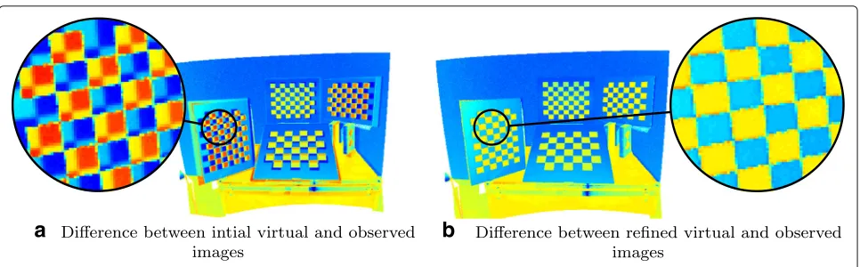
In Fig. 3a, double edges at the checkerboard quads indicate that the two images are not accurately aligned. Figure 3b shows the difference image of the Kinect’s
Table 1Mean calibration error and standard deviation for four cameras in 2-D and 3-D for two calibration approaches
Camera ICP 2-D (px) Proposed 2-D (px) ICP 3-D (cm) Proposed 3-D (cm)
Kinect V2 1.172±0.492 0.176±0.084 1.113±0.108 0.267±0.064
CamBoard Pico Flexx 2.309±0.509 0.305±0.125 0.930±0.124 0.319±0.134
Astra 0.491±0.232 0.418±0.119 1.135±0.444 0.126±0.038
a
b
Fig. 3Impact of refinement for the calibration scene and the Kinect V2.aDifference between the virtual reflectance image and the observed image. Inaccuracies in the initialization cause edges to appear twice.bDifference image between the final reflectance image and the amplitude image of the camera: all edges accurately coincide
amplitude image and the virtual reflectance image after refinement. In the refined result, no double edges can be observed. Instead, all checkerboard quads as well as the borders of the pattern boards are accurately aligned.
4.5 Range camera evaluation
For this experiment, we use the calibration results to generate ground truth distance data for the three general scenes. Depending on the focus of the study, the scenes have to be designed differently. The primary interest of the following experiment is to evaluate the absolute measurement accuracy of the range cameras with a certain volume of interest. Furthermore, we set up the scene such that several char-acteristics of the different range camera technologies can be illustrated. In this evaluation, we present as an example evaluation results for the Kinect V2 and the RealSense R200 camera, i.e, representatives of both classes of range cameras.
The setup consists of several objects which are posi-tioned in front of the sensors: boxes, cylinders, etc. Each scene is captured first with the laser scanner then with the two cameras, to exclude mutual interference. Then, the individual range camera measurements are compared to the reference distance images which have been generated from laser scanner data. For visualizing the measurement errors, we subtract the observed distance image from the virtual distance image.
In Fig. 4 we demonstrate some of the characteristic properties of each sensor type on one of the general scenes. To investigate the dependency of measurement error and distance, we combine the result of the three gen-eral scenes and plot the errors for a region of interest as shown in Fig. 5. The mean accuracy is calculated for 1-cm bins and plotted in black. Gray dots represent individual measurements.
4.5.1 Kinect V2
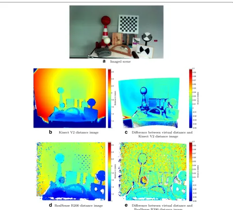
The ToF sensor provides dense distance measurements for all pixels which are properly illuminated (see Fig. 4b). In Fig. 4c, the measurement errors for all pixels which lie in the common field of view of the laser scanner and the range camera are illustrated. Two characteristic errors can be observed in this figure: an amplitude-dependent error and multi-path effects [7]. The amplitude-dependent error can be observed best in the lower right cor-ner of the image in the area of the calibration target. Even though the surface of this target is flat, a clear change of distances can be observed between high- and low-reflectivity regions. Multi-path can be observed best in the central image region. In this area, the emitted light can easily hit multiple regions one after another before being reflected back to the camera. Especially for pixels that belong to the flat surface of the box, the acute view-ing angle fosters a comparably large impact of multi-path effects.
a
b c
d e
Fig. 4Per-pixel accuracy evaluation for one of the general scenes. Distances and measurement errors are given in meters and encoded as colors. aImaged scene.bKinect V2 distance imagecdepth error for Kinect V2.dRealSense R200 distance image.edepth error for RealSense R200
4.5.2 RealSense R200
In this section, characteristic errors of the RealSense R200 structured light camera are investigated. Stereo block matching and the subsequent internal processing causes the speckle-like pattern that can be observed best in the planar background region of Fig. 4e. Block matching also causes fringes at sharp borders, e.g., at the borders of the spheres. Similarly as the time-of-flight camera, this sen-sor also relies on the requirement that the emitted light is reflected back to the cameras. If the imaged surface does not reflect the light in the spectrum of the emitter, then no or only inaccurate measurements are possible. These effects can be observed in the lower left sphere (inaccurate
measurements) and at the lower right calibration target. A characteristic of structured-light cameras is that the base-line between projector and observing camera introduces occluded image regions, seen best at the disc on the right side of the image.
a
b
c
d
g
h
e
f
Fig. 5Measurement error with respect to distance.a–cEvaluated ROI of the three scenes from the perspective of the Kinect V2 camera. d–fRespective ROIs for the RealSense R200 sensor.g,hMean measurement error with respect to distance. Gray dots depict individual
measurements. The black line represents the mean measurement error within 1 cm. The red line marks the zero-level to help reading the plots. The light blue overlays highlight interesting distance ranges which are discussed in the evaluation. (Kinect V2: 1.5 to 1.85 m, RealSense R200: 1.8 to 2.3 m)
5 Conclusion
We presented a novel method for finding the spatial rela-tion between a camera and laser scanner based on stereo calibration. The algorithm enables the user to calibrate the laser scanner to a camera with high accuracy using only a single shot of a calibration scene.
In our evaluation, we compare the proposed method to a similar, calibration pattern-based approach and show that our method achieves notably more accurate calibration
The applicability of the method is demonstrated in the context of range camera evaluation. Here, we use the method to investigate the measurement errors of a time-of-flight and a structured light camera: the Microsoft Kinect V2 and the Intel RealSense R200. In this evalu-ation, we can showcase several error sources which are characteristic to the different range sensing technologies.
Acknowledgements
We thank PMD technologies for providing the Camboard Pico Flexx time-of-flight camera which has been used in this evaluation.
Authors’ contributions
PF performed the primary development of the algorithm, designed the evaluation, and wrote the intial draft of the manuscript. CP helped with the data acquisition and provided the laser scanner. AM and CR supervised the work. CR also played an essential role in drafting and refining the final manuscript. All authors read and approved the manuscript.
Competing interests
The authors declare that they have no competing interests.
Publisher’s Note
Springer Nature remains neutral with regard to jurisdictional claims in published maps and institutional affiliations.
Author details
1Pattern Recognition Lab, University of Erlangen - Nuremberg, Martensstrasse
3, Erlangen, Germany.2Metrilus GmbH, Henkestrasse 91, Erlangen, Germany.
3Ostbayerische Technische Hochschule Regensburg, Pruefeninger Strasse 58,
Regensburg, Germany.
Received: 31 March 2017 Accepted: 18 October 2017
References
1. Buck S, Hanten R, Bohlmann K, Zell A (2016) Generic 3D obstacle detection for AGVs using time-of-flight cameras. In: 2016 IEEE/RSJ International Conference on Intelligent Robots and Systems (IROS). pp 4119–4124 2. Smith T (2016) Astrobee: A New Platform for Free-Flying Robotics on the
International Space Station. In: Proceedings of the International Symposium on Artificial Intelligence, Robotics and Automation in Space (i-SAIRAS 2016)
3. Klionovska K, Benninghoff H (2017) Initial Pose Estimation using PMD Sensor during the Rendezvous Phase in On-Orbit Servicing Missions. In: 27th AAS/AIAA Space Flight Mechanics Meeting
4. Leo M, Natale A, Del-Coco M, Carcagnì P, Distante C (2017) Robust Estimation of Object Dimensions and External Defect Detection with a Low-Cost Sensor. J Nondestruct Eval 36(1)
5. Rauscher G, Dube D, Zell A (2014) A Comparison of 3D Sensors for Wheeled Mobile Robots. In: 2014 International Conference on Intelligent Autonomous Systems (IAS-13). Padova
6. Yang L, Zhang L, Dong H, Alelaiwi A, Saddik AE (2015) Evaluating and Improving the Depth Accuracy of Kinect for Windows v2. EEE Sensors J 15(8):4275–4285
7. Fuersattel P, Placht S, Balda M, Schaller C, Hofmann H, Maier A, et al. (2016) A Comparative Error Analysis of Current Time-of-Flight Sensors. IEEE Trans Comput Imaging 2(1):27–41
8. Wasenmüller O, Stricker D (2017) Comparison of Kinect v1 and v2 Depth Images in Terms of Accuracy and Precision. In: Asian Conference on Computer Vision Workshop Asian Conference on Computer Vision Workshop (ACCV)
9. Nair R, Meister S, Lambers M, Balda M, Hofmann H, Kolb A, et al. (2013) Ground Truth for Evaluating Time of Flight Imaging. In: Time-of-Flight and depth imaging: Sensors, algorithms, and applications : Dagstuhl 2012 Seminar on Time-of-Flight Imaging and GCPR 2013 Workshop on Imaging New Modalities. pp 52–74
10. Zhang Q, Pless R (2004) Extrinsic calibration of a camera and laser range finder (improves camera calibration). In: 2004 IEEE/RSJ International Conference on Intelligent Robots and Systems (IROS). pp 2301–2306
11. Kassir A, Peynot T (2010) Reliable automatic camera-laser calibration. In: Proceedings of the 2010 Australasian Conference on Robotics & Automation
12. Zhou L (2014) A New Minimal Solution for the Extrinsic Calibration of a 2D LIDAR and a Camera Using Three Plane-Line Correspondences. IEEE Sensors J 14(2):442–454
13. Unnikrishnan R, Hebert M (2005) Fast Extrinsic Calibration of a Laser Rangefinder to a Camera. Pittsburgh
14. Geiger A, Moosmann F, Car O, Schuster B (2012) Automatic camera and range sensor calibration using a single shot. In: 2012 IEEE International Conference on Robotics and Automation (ICRA). pp 3936–3943 15. Ha JE (2012) Extrinsic calibration of a camera and laser range finder using
a new calibration structure of a plane with a triangular hole. Int J Control Autom Syst 10(6):1240–1244
16. Hoang VD, Cá D, Jo KH (2014) Simple and Efficient Method for Calibration of a Camera and 2D Laser Rangefinder. In: Hutchison D, Kanade T, Kittler J, Kleinberg JM, Mattern F, Mitchell JC, et al (eds). Intelligent Information and Database Systems, vol 8397 of Lecture Notes in Computer Science. Springer International Publishing. pp 561–570
17. Gong X, Lin Y, Liu J (2013) 3D LIDAR-camera extrinsic calibration using an arbitrary trihedron. Sensors 13(2):1902–1918
18. Moghadam P, Bosse M, Zlot R (2013) Line-based extrinsic calibration of range and image sensors. In: 2013 IEEE International Conference on Robotics and Automation (ICRA). pp 3685–3691
19. Taylor Z, Nieto J (2012) A Mutual Information Approach to Automatic Calibration of Camera and Lidar in Natural Environments. In: Proceedings of Australasian Conference on Robotics and Automation (ACRA). pp 31–39 20. Taylor Z, Nieto J (2013) Automatic calibration of lidar and camera images
using normalized mutual information. University of Sydney, Australia 21. Pandey G, McBride JR, Savarese S, Eustice RM (2015) Automatic Extrinsic
Calibration of Vision and Lidar by Maximizing Mutual Information. J Field Robot 32(5):696–722
22. Levinson J, Thrun S (2013) Automatic Online Calibration of Cameras and Lasers. In: Proceedings of Robotics: Science and Systems. Berlin 23. Scott T, Morye AA, Pinies P, Paz LM, Posner I, Newman P (2015) Exploiting
known unknowns: Scene induced cross-calibration of lidar-stereo systems. In: 2015 IEEE/RSJ International Conference on Intelligent Robots and Systems (IROS). pp 3647–3653
24. Poppinga J, Vaskevicius N, Birk A, Pathak K (2008) Fast plane detection and polygonalization in noisy 3D range images. In: 2008 IEEE/RSJ International Conference on Intelligent Robots and Systems. pp 3378–3383
25. Holz D, Behnke S (2014) Approximate triangulation and region growing for efficient segmentation and smoothing of range images. Robot Auton Syst 62(9):1282–1293
26. Placht S, Fürsattel P, Mengue EA, Hofmann H, Schaller C, Balda M, et al. (2014) ROCHADE: Robust Checkerboard Advanced Detection for Camera Calibration. In: Fleet D, Pajdla T, Schiele B, Tuytelaars T (eds). Computer Vision – ECCV 2014. vol. 8692 of Lecture Notes in Computer Science. Springer International Publishing, Cham. pp 766–779
27. Horn BKP (1987) Closed-form solution of absolute orientation using unit quaternions. J Opt Soc Am A 4(4):629–642
28. Zhang Z (2000) A flexible new technique for camera calibration. IEEE Trans Pattern Anal Mach Intell 22(11):1330–1334