Detection and Classification of Normal and Abnormal Heart Diseases Using SIFT and SVM

(1)

183901-5757-IJVIPNS-IJENS © February 2018 IJENS _{I J E N S}

Detection and Classification of Normal and Abnormal

Heart Diseases Using SIFT and SVM

Dr. M. Balasubramanian, M. JannathlFirdouse, Student

Member, IEEE

Abstract— The lung cancer only accounts more deaths than any other type of cancers in both men and women. Lung zones are identified by assessing the lungs by comparing the upper, middle and lower lung parts on the left and right. Asymmetry of lung density is denoted as either abnormal whiteness (increased densi-ty), or abnormal blackness (decreased density). Once the asym-metry is spotted, the next step is to decide which side is abnor-mal. If there is an area that is different from the surrounding is bilateral lung, then this is likely to be the abnormal area. If the alveoli and small airways fill with dense material, the lung is said to be consolidated. The early detection of lung cancer makes the survival rate of patients. In this paper, we proposed a method for the detection and classification of chest images using Scale Invar-iant Feature Transform and Support Vector Machine. The SIFT descriptor detects the key points from the gray level images. Sev-en features are detected by applying the SVM principle with SIFT transform. The performance measures such as precision, recall, accuracy and F-Score are estimated. We have collected more than 100 CT images for this classification from Radiological center, KIMS Hospital. The normal and abnormal chest images are classified with the better performance measures.

Index Term— SIFT, SVM, Normal and abnormal images, Pre-cision, Recall, F-Score

1. INTRODUCTION

The genuine lung cancers are the most comprehensively studied tumors of the lung. This accounts for one third of can-cer deaths in the world wide. The lung cancan-cers are classified in to two types. They are small cell lung cancer and non-small cell lung cancer. Non-small cell lung cancer is further classi-fied in to Adeno50%, Squamous cell carcinoma-35% and large cell lung cancer-15%. Also the other types adeno-squamous carcinoma and sarcomatoid carcinoma. It is important to be aware that consolidation does not always mean there is infection, and the small airways may fill with material other than pus as in pneumonia, such as fluid like pulmonary oedema, blood like pulmonary haemorrhage, or cells which causes cancer. They all look similar and clinical information will often help to decide the diagnosis. The area of lung becomes dense and white when it is consolidated. If the larger airways are out of danger, they are of relatively low density which should be in blacker. This phenomenon is known as air bronchogram and it is a characteristic sign of

consolidation shown in figure 1.

Fig. 1.Consolidation with air bronchogram

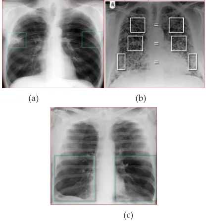
The following figures 2(a) to (c) describes about the small lung zone abnormalities and bilateral lung abnormalities in details. The careful comparison of the lung zones can lead to noticing smaller abnormalities which may otherwise be ignored. Comparing sides does not always give the answer. The lungs may be abnormal on both sides and so awareness of the normal appearances of lung parenchyma becomes more important. The abnormal lung is identified when there is asymmetry of the lungs, sometimes it is the dark which is the less dense.

(a) (b)

(c)

Fig. 2. (a) Unilateral middle zone abnormality (b) Bilaterally Abnormal Lung Zones (c) Unilateral Black Lower Zone

It is generally best to refer to the location of lung ab-normalities in terms of zones, occasionally you will see signs ————————————————

 Dr. M. Balasubramanian, Department of Computer Science and Engi-neering, Annmalai University, Kadallore. E-mail:

[email protected]

 M. Jannathl Firdouse, Research Scholar, Research and Development Center, Bharathiyar University, Coimbatore. E-mail:

(2)

that will tell you which specific lobe is involved. The right middle lobe is bordered medially by the right heart border and superiorly by the horizontal fissure. Any abnormality, which increases density of this lobe, may therefore obscure the right heart border, or be limited superiorly by the horizontal fissure.

Another indicator of the location of pathology may be the displacement of the horizontal fissure. May be because of volume loss of the right upper lobe, for example due to col-lapse, or fibrosis, the fissure is displaced upwards. There may be a process which has caused volume loss of the right lower lobe and then the horizontal fissure is displaced down-wards.Figures 3(a) and (b) shows the frontal and lateral view of left lower lobe.The major (or oblique) fissures cannot be identified on a frontal chest X-ray. This is because they are oriented obliquely en-face. A lateral view can demonstrate if a lung abnormality is anterior or posterior to the major fissures.

Fig. 3. (a) Left lower lobe cavity (b) Left lower lobe cavity - frontal view - lateral view

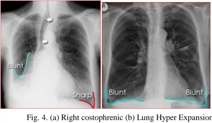
The blunting of the costophrenic angles is usually caused by a pleural effusion. Other causes of costophrenic angle blunting include lung disease in the region of the costophrenic angle, and lung hyper expansion. Both costophrenic angles are blunt due to lung hyper-expansion. The hemi-diaphragms are flat-tened indicating hyper-expansion. The lung markings are dis-torted bilaterally as shown in figure 4 (a) and (b).

Fig. 4. (a) Right costophrenic (b) Lung Hyper Expansion angle blunting

The lungs are normal. The diaphragm is crisply defined on both sides (arrowheads) Air under the diaphragm (asterisks) is seen as crescents of relatively low density (black) Black air can be seen on both sides of the bowel wall (blue line) – this is known as the double-wall sign or Rigler's sign (usually only seen on abdominal X-rays). The clinical information are acute, severe abdominal pain, abdominal guarding on examination and risk factors for peptic ulceration included smoking, high alcohol intake, and long term use of non-steroidal anti-inflammatory drugs.

(3)

2 FEATURE EXTRACTION

In image processing, feature extraction is a special form of dimensionality reduction. When the input data to an algorithm is too large to be processed and it is suspected to be very redundant, then the input data will be transformed into a reduced representation set of features (also named features vector) [7]. Transforming the input data into the set of features is called feature extraction. If the features extracted are care-fully chosen it is expected that the features set will extract the relevant information from the input data in order to perform the desired task using this reduced representation instead of the full size input.

2.1 Scale Invariant Feature Transform (SIFT)

Scale-invariant feature transform (or SIFT) is an al-gorithm [8] to detect and describe local features in images. The algorithm was published by David Lowe. SIFT can ro-bustly identify objects even among clutter and under partial occlusion, because the SIFT feature descriptor is invariant to uniform scaling, orientation, and partially invariant to affine distortion and illumination changes. The SIFT descriptor comprised a method for detecting interest points from a grey-level image at which statistics of local gradient directions of image intensities were accumulated to give a summarizing description of the local image structures in a local neighbor-hood around each interest point.

The four real stages to catch the peculiarity portrayal of a picture are:

 Detection of scale-space Extrema

 Keypoint localization

 Orientation assignment

 Keypoint descriptor

2.1.1. Detection of scale-space extrema

The first stage is to construct a Gaussian "scale space" function from the input image. This is formed by con-volution of the original image with Gaussian functions of var-ying widths.The scale space of an image is defined as a func-tion L(x,y,𝜎) that isproduced from the convolution of a vari-able-scale Gaussian, G(x,y,𝜎) with an input image, I(x,y):

L(x,y, 𝜎) = G(x,y, 𝜎) ∗ I(x,y)---(1)

Where ‘∗’ is the convolution operation in x and y, and

G(x,y,𝜎)= 1 2πσ2𝑒

−(x2+y2)/2σ2_{--- (2)}

To efficiently detect stable keypoint locations in scale space, Lowe proposed using scale-space extrema in the

differ-ence-of-Gaussian function convolved with the image, D(x, y,

), which can be computed from the difference of two nearby scales separated by a constant multiplicative factor k:

DoG (x, y,σ ) =(G(x,y,kσ) − G(x, y, σ)) ∗ I(x,y)

=L(x, y, k𝜎) −L(x, y, 𝜎) --- (3)

There are a number of reasons for choosing this func-tion. First, it is a particularly efficient function to compute, as the smoothed images, L, need to be computed in any case for scale space feature description, and DoG can therefore be computed by simple image subtraction. To detect the local maxima and minima of DoG(x, y, σ) each point is compared with its 8 neighbours at the same scale, and its 9 neighbours up and down one scale. If this value is the minimum or maxi-mum of all these points then this point is an extrema.

2.1.2 Key point Localization

This stage attempts to eliminate some points from the candidate list of keypoints by finding those that have low con-trast or are poorly localised on an edge. The value of the key-points in the DoG pyramid at the extrema is given by:

D (z) = D + 1 2

∂D−1

∂x 𝑧--- (4)

If the function value at z is below a threshold value this point is excluded.

To eliminate poorly localisedextrema we use the fact that in these cases there is a large principle curvature across the edge but a small curvature in the perpendicular direction in the difference of Gaussian function. A 2x2 Hessian matrix, H, computed at the location and scale of the keypoints is used to find the curvature. With these formulas, the ratio of principal curvature can be checked efficiently.

H= [Dxx Dxy

Dxy Dyy]--- (5)

2.1.3 Orientation Assignment

This step aims to assign a consistent orientation to the keypoints based on local image properties. An orientation histogram is formed from the gradient orientations of sample points within a region around the keypoints. A 16x16 square is chosen in this implementation. The orientation histogram has 36 bins covering the 360 degree range of orientations. The gradient magnitude, m(x, y), and orientation, θ(x, y), are pre-computed using pixel differences:

m(x,y)=

√(L(x + 1, y) − L(x − 1, y))2 + (L(x, y + 1) − L(x, y − 1))2

(4)

θ(x, y) = tan−1₍L(x,y+1)−L(x,y−1)

L(x+1,y)−L(x−1,y))---(7) Each sample is weighted by its gradient magnitude and by a Gaussian-weighted circular window with an σ that is 1.5 times that of the scale of the keypoints. Peaks in the orien-tation histogram correspond to dominant directions of local gradients. We locate the highest peak in the histogram and use this peak and any other local peak within 80% of the height of this peak to create a keypoints with that orientation. Some points will be assigned multiple orientations if there are multi-ple peaks of similar magnitude. A Gaussian distribution is fit to the 3 histogram values closest to each peak to interpolate the peaks position for better accuracy. This computes the loca-tion, orientation and scale of SIFT features that have been found in the image. These features respond strongly to the corners and intensity gradients. The length of the arrows indi-cates the magnitude of the contrast at the keypoints, and the arrows point from the dark to the bright side.

2.1.4 Key-point Descriptor

In this stage, a descriptor is computed for the local image region that is as distinctive as possible at each candidate keypoint [9]. The image gradient magnitudes and orientations are sampled around the keypoint location. A Gaussian weighting function with σ related to the scale of the keypoint is used to assign a weight to the magnitude. We use an σ equal to one half the width of the descriptor window in this imple-mentation. In order to achieve orientation invariance, the co-ordinates of the descriptor and the gradient orientations are rotated relative to the keypoint orientation [10]. This process is indicated in figure 5 a 16x16 sample array is computed and a histogram with 8 bins is used. So a descriptor contains 16x16x8 elements in total.

Fig. 5. Building key-point

These are weighted by a Gaussian window, indicated by the Overlaid circle. The image gradients are added to an orientation histogram. Each Histogram include 8 directions indicated by the arrows and is computed from 4x4 Sub re-gions. The length of each arrow corresponds to the sum of the gradient magnitudes near that direction within the region.

3 RECOGNITION OF INDOOR OBJECTS USING SVM

Support vector machine [11], [12] is based on the principle of structural risk minimization (SRM). Like RBFNN, support vector machines can be used for pattern clas-sification and nonlinear regression. SVM constructs a linear

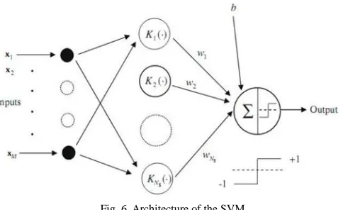
model to estimate the decision function using non-linear class boundaries based on support vectors. If the data are linearly separated, SVM trains linear machines for an optimal hyper plane that separates the data without error and into the maxi-mum distance between the hyper plane and the closest training points. The training points that are closest to the optimal sepa-rating hyper plane are called support vectors. Figure 6 shows the architecture of the SVM. SVM maps the input patterns into a higher dimensional feature space through some nonline-ar mapping chosen a priori. A linenonline-ar decision surface is then constructed in this high dimensional feature space. Thus, SVM is a linear classifier in the parameter space, but it becomes a nonlinear classifier as a result of the nonlinear mapping of the space of the input patterns into the high dimensional feature space.

3.1 SVM Principle

Support vector machine (SVM) ban be used for clas-sifying the obtained data (Burges, 1998). SVM are a set of related supervised learning methods used for classification and regression. They belong to a family of generalized linear clas-sifiers. Let us denote a feature vector (termed as pattern) by x=(x1, x2, · · ·,xn) and its class label by y such that y = {+1, −1}. Therefore, consider the problem of separating the set of n-training patterns belonging to two classes.

Fig. 6. Architecture of the SVM

A decision function g(x) that can correctly classify an input pattern x that is not necessarily from the training set.

3.2 SVM for Linearly Separable Data

A linear SVM is used to classify data sets which are linearly separable. The SVM linear classifier tries to maximize the margin between the separating hyper planes. The patterns lying on the maximal margins are called support vectors. Such a hyper plane with maximum margin is called maximum mar-gin hyper plane. In case of linear SVM, the discriminate func-tion is of the form:

g (x) = ωt_{x + b --- --- (8)}

(5)

classes are separated by the hyperplane g (x) = 𝜔t_{x+b =0.} SVM finds the hyper plane that causes the largest separation between the decision function values from the two classes. Mathematically, this hyper plane can be found by minimizing the following cost function:

j (ω) = ωt ω_---(9)

For the linearly separable case, the decision rules de-fined by an optimal hyper plane separating the binary decision classes are given in the following equation in terms of the support vectors:

Y = sign (∑i=N_{i=1 i}y (xxi) + b) --- (10)

where Y is the outcome, yiis the class value of the training example xi and represents the inner product [13], [14]. The vector corresponds to an input and the vectors xi, i = 1. . .Ns, are the support vectors.

3.3 SVM for Linearly Non- Separable Data

For non-linearly separable data, it maps the data in the input space into a high dimension space with kernel function

(x), to find the separating hyper plane.

Y = sign (∑i=N_{i=1 i}y k(xx_i) + b) --- (11)

3.4 Determining Support Vectors

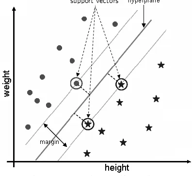
The support vectors are the (transformed) training pat-terns. The support vectors are (equally) close to hyper plane. The support vectors are training samples that define the opti-mal separating hyper plane and are the most difficult patterns to classify. Informally speaking, they are the patterns most informative for the classification task. Figure 7 shows a SVM example to classify a person into two classes: overweighed, not overweighed; two features are pre-defined: weight and height. Each point represents a person. Dark circle and star points denote overweighed and not overweighed respectively. Circles over the points as shown in figure 7 denote support vectors.

Fig. 7. SVM example to classify two classes

3.5 Inner Product Kernels

SVM generally applies to linear boundaries. In the case where a linear boundary is inappropriate SVM can map

the input vector into a high dimensional feature space. By choosing a non-linear mapping, the SVM constructs an opti-mal separating hyperplane in this higher dimensional space, as shown in figure 8. The function K is defined as the kernel function for generating the inner products to construct ma-chines with different types of non-linear decision surfaces in the input space.

K (x, xi) =  (x).  (xi) --- (12)

The kernel function may be any of the symmetric functions that satisfy the Mercer’sConditions. There are sever-al SVM kernel functions as given in Table I.

Table I

Types of SVM inner product kernels

Types of Ker-nels

Inner Product Kernel k(xT_,x_i₎

Details

Polynomial (xT_x_i_{+ 1)}p

Where x is

input

pat-terns, xi is

support vec-tors, 2 is

var-iance, 1≤ 𝑖 ≤

𝑁s, Ns is

number of

support vec-tors, 0,1 are constant val-ues. P is de-gree of the polynomial Gaussian Exp[-||xT_-

xi||2/22]

Sigmoidal Tan h (0xT_x_i₊ 1)

The various types of SVM inner product kernels are shown in table Isuch as Polynomial, Gaussian and sigmoidal Kernels.

Fig. 8. An example for SVM kernel function (a) Non-linear problem. (b) Linear problem

4 EXPERIMENTAL RESULTS

(6)

rithm. From the captured images, indoor objects were recog-nized.

4.1 SIFT Features with SVM

In training phase, SIFT is applied to all object catego-ries. In our work 7 features are extracted from each keypoint by using SIFT features. Number of pixels extracted from an input image is differ from image to image, as well as depends on the complexity of an image. The seven features are x posi-tion, y posiposi-tion, scale(sub-level), size of feature on image, edge flag, edge orientation, curvature of response through scale space. SIFT performs Extra ordinarily robust matching technique. It can handle changes in viewpoint, it can handle significant changes in illumination, and it is fastand efficient and can run in real time.

In testing phase, SIFT is applied to the test sample [15] and depends upon the complexity of an image it extract the keypoints, ineach keypoint7 features are extracted. SVM recognize the heart disease (or normal heart image) image by using the test features compared with train features of differ-ent heart disease and normal chest images. The detection per-formance is evaluated using the heart diseases dataset which consists of 20 normal chest images and 20diseased chest im-ages.

4.2 Performance Measures

The correctness of a classification can be evaluated by computing the number of correctly recognized class exam-ples (true positives), the number of correctly recognized ex-amples that do not belong to the class (true negatives), and examples that either were incorrectly assigned to the class (false positives) or that were not recognized as class examples (false negatives).

4.2.1 Precision

Precision is a measure of the accuracy provided that a specific class has been predicted. It is defined by:

Precision=_{number of true positive+false positives}number of true positive ----(13)

4.2.2 Recall

Recall is a measure of the ability of a prediction model to select instances of a certain class from a data set. It is commonly also called sensitivity, and corresponds to the true positive rate. It is defined by the formula:

Recall= number of true positives

number of true positives +false negatives---(14)

4.2.3 Accuracy

Accuracy is the overall correctness of the model and is calculated as the sum of correct classifications divided by the total number of classifications.

Accuracy=

number of true positive + true negative

number of true positive + false negative + false positive + true negative -- (15)

4.2.4 F-score

A measure that combines precision and recall is the harmonic mean of precision and recall, the traditional f-measure or balanced f-score:

F-score =2∗precision∗recall

precision+recall---(16)

Table II

Confusion matrix for detection of normal and diseased heart with SIFT using SVM

The Confusion matrix for detection of normal and diseased heart with SIFT using SVM is shown in Table II.

Fig. 9.chart represents the overall performance of detection of normal and diseased heartfrom database with SIFT using SVM

The chart that represents the performance of detec-tion of normal and diseased heart from database with SIFT using SVM is shown in figure 9.

Table III

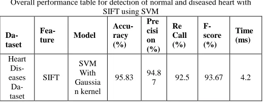
Overall performance table for detection of normal and diseased heart with SIFT using SVM

Da-taset

Fea-ture Model

Accu-racy (%)

Pre cisi on (%)

Re Call (%)

F-score (%)

Time (ms)

Heart Dis-eases

Da-taset

SIFT

SVM With Gaussia n kernel

95.83 94.8

7 92.5 93.67 4.2

Overall performance table for detection of normal and dis-10

20 30 40 50 60 70 80 90 100

Lung Deseased Data Set

Data Set Heart Type

TP FN FP TN

Normal Heart 19 1 1 39

Abnormal

(7)

eased heart is shown in tableIII.

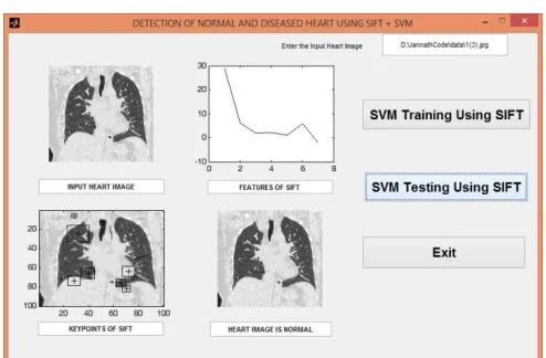
4.3 Screen Shots

Fig.10. Screen shot for Detection of Normal Heart Using SIFT and SVM

Fig. 11. Screen shot for Detection of Diseased Heart Using SIFT and SVM

Figures 10 and 11 show the screen shots for Detection of Normal and Diseased Heart Using SIFT and SVM respective-ly.

5 CONCLUSION AND FUTURE ENHANCEMENT

A method for detection and classification normal and abnormal chest images was presented. An approach for feature extraction using SIFT from normal and abnormal chest images and classification of normal and abnormal chest images using SVM have been proposed and implemented. Seven features were extracted from each point using SIFT features. Finally, the chest images are classified (normal/abnormal) using SVM. The performance of the system achieves an accuracy rate about 95.83 % using SIFT and SVM. In future work, a new feature extraction techniquewill beproposed to detect and

classify normal and abnormal chest images and to improve the performance of the system.

REFERENCES

[1] F. B. J. M. Thunnissen, “Sputum examination for early Detection of lung cancer”, J.Clin.Pathol. vol. 56, no. 11, pp. 805– 810, Nov. 2003.

[2] J. Priyadharshini and M.S. Sridhonkar, “Detection of Lung Cancer using SVM Classification”, International Research Journal of En-gineering and Technology, vol. 4, Issue 6, pp. 378 – 381, June 2017.

[3] S. Dua, V. Jain, and H; W; Thompson, “Patient classification us-ing association minus-ing of clinicalimages”, in 5th IEEE Interna-tional Symposium on Biomedical Imaging: From Nano to Macro, ISBI 2008, pp.253– 256, 2008.

[4] I. Sluimer, A. Schilham, M. Prokop, and B. Van Ginneken, “Com-puter analysis of computed tomography scans of the lung: a sur-vey”, IEEE Transaction on Medical Imaging, vol. 25, no.4, pp. 385– 405, 2006.

[5] F. Taher, N. Werghi, and H. Al-Ahmad, “Comparison of Hopfield Neural Network and Mean Shift algorithm in Segmenting Sputum Color Images for Lung Cancer Diagnosis”, in 20th IEEE Interna-tional Conference on Electronics, Circuits, and Systems (ICECS), Abu Dhabi, UAE, pp. 649– 652, 2013.

[6] F. Taher, N. Werghi, H. Al-Ahmad, and C. Donner, “Extraction and Segmentation of Sputum Cells for Lung Cancer Early Diagnosis”, Algorithms, vol. 6, No. 3, pp. 512– 531, Aug. 2013.

[7] Y. P. Chien, K. S. Fu, "Recognition of X-ray picture pat-terns", IEEE Trans. Syst. Man Cybern., vol. SMC-4, No. 2, pp. 145-156, Mar. 1974.

[8] E. L. Hall, R. P. Kruger, S. J. Dwyer, D. L. Hall, R. W. McLaren, G. S. Lodwick, "A survey of pre-processing and feature extraction techniques for radiographic images", IEEE Trans. Comput., vol. C-20, no. 9, pp. 1032-1044, Sept. 1971.

[9] J. Fridrich (1999) "Methods for Tamper Detection in Digital

Imag-es". In Proc. of ACM Workshop on Multimedia and Security, Or-lando, FL, pp.19-23.

[10] Regina Lionnie, Rizal BroerBahaweres, Said Attamimi,

MudrikAlaydrus, “A Study on Pre-Processing Methods for Copy-Move Forgery Detection Based on SIFT”, Region 10, Conference TENCON 2017 – IEEE, pp.1142 – 1147, 2017, ISSN 2159-3450

[11] V. Vapnik, Statistical Learning Theory, John Wiley and Sons, New York, 1998.

[12] J.C. Burges Christopher, “A tutorial on support vector machines for pattern recognition”, Data mining and knowledge discovery, vol. 52, pp. 121–167, 1998.

[13] B. Heisele, P. Ho, and T. Poggio, “Face recognition with support vector machines: Global versus component-based approach”, in Proc. 8th Int. Conf. Computer Vision, Vancouver, BC, Canada, 2001, pp. 688–694.

[14] B. Heisele, Alessandro, and T. Poggio, “Learning and vision ma-chines”, Proc. IEEE, vol. 90, no. 7, pp. 1164–1177, July 2002. [15] S. Sathiya, M. Balasubramanian, S. Palanivel, “Pattern

Recogni-tion Based DetecRecogni-tion RecogniRecogni-tion of Traffic Sign Using SVM”, In-ternational Journal of Engineering and Technology (IJET), Vol 6, No 2, pp: 1147 – 1157, Apr-May 2014

ACKNOWLEDGMENT

(8)

BIBLIOGRAPHY

Dr. M. Balasubramanian received his B.E degree in Computer Science and Engineering from Government College of Engineering (GCE), Tirunelveli in the year 1996. He re-ceived his M.Tech degree in Computer Appli-cations from Indian Institute of Technology, Delhi in the year 2004. He has been with An-namalai University, since 1999. He received Ph.D in Computer Science and Engineering from Annamalai University in the year 2011. He published papers in 30 international journals and conferences. He received Career Award for Young Teachers (CAYT) from All India Council for Technical Education (AICTE), New Delhi. He is the Co-Investigator of an UGC Major Research project since 2012. He has organized workshops in the field of image and speech processing, and Latex. He has delivered special lectures in several topics of his area, in workshops and staff development programme. Currently, six research scholars are pursuing research under his guidance in the area of image and video processing. His research interest includes image and video processing, pattern classification and neural networks.