Machine Learning Pipeline for Exoplanet
Classification
George Clayton Sturrock
Southern Methodist University, [email protected]
Brychan Manry
Southern Methodist University, [email protected]
Sohail Rafiqi
Southern Methodist University, [email protected]
Follow this and additional works at:
https://scholar.smu.edu/datasciencereview
Part of the
Applied Statistics Commons
,
Artificial Intelligence and Robotics Commons
,
Other
Astrophysics and Astronomy Commons
,
Probability Commons
,
Stars, Interstellar Medium and the
Galaxy Commons
, and the
Theory and Algorithms Commons
Recommended Citation
Sturrock, George Clayton; Manry, Brychan; and Rafiqi, Sohail (2019) "Machine Learning Pipeline for Exoplanet Classification,"SMU Data Science Review: Vol. 2 : No. 1 , Article 9.
Machine Learning Pipeline for Exoplanet Classification
Brychan Manry, George Sturrock, Sohail RafiqiMaster of Science in Data Science, Southern Methodist University, Dallas, TX 75275 USA
{bmanry, gsturrock, srafiqi}@smu.edu
Abstract. Planet identification has typically been a tasked performed exclusively by teams of astronomers and astrophysicists using methods and tools accessible only to those with
years of academic education and training. NASA’s Exoplanet Exploration program has introduced modern satellites capable of capturing a vast array of data regarding celestial objects of interest to assist with researching these objects. The availability of satellite data has opened up the task of planet identification to individuals capable of writing and interpreting machine learning models. In this study, several classification models and datasets are utilized to assign a probability of an observation being an exoplanet. A Random Forest Classifier was selected as the optimum machine learning model to classify objects of interest in the Cumulative Kepler Object of Information table. The Random Forest Classifier obtained a cross-validated accuracy score of 98%. 968 candidate observations have a greater than 95% probability of being an exoplanet. Finally, the Random Forest Classifier was made publicly accessible by an application programming interface (API) and an Azure Container Instance web service in the Microsoft Azure cloud.
1 Introduction
Astronomy is one of human civilization’s oldest natural sciences. Throughout history, astronomy has influenced religion, guided explorers, defined food production schedules and fueled philosophical questions surrounding our very existence and role in the universe1. A natural extension of our curiosity with the stars is to question if there is another planet, in another solar system capable of supporting life. The answer to this question has been pondered and researched for hundreds of years.
The task of identifying planets outside of our solar system, known as exoplanets, leads to genuinely novel discoveries. Exoplanet identification has traditionally been a time-intensive task reserved for highly-trained, educated experts with access to specialized—and usually expensive—equipment. These experts relied upon their education, intelligence, diligence, and team knowledge in their painstaking search for exoplanets using images collected by terrestrial observatories and satellite-based telescopes, such as Hubble.
A new era has dawned in the hunt for exoplanets however; a new generation of modern satellites, such as Kepler, have been launched in recent years with the goal of partially automating scientific observations and data generation related to exoplanet identification. These satellites are engineered to not only take pictures but to process those images using proven astronomical techniques to produce a vast collection data with the right variety of features for
identifying exoplanets. Astronomers and physicists can interrogate this data to help confirm if an object of interest they have discovered is indeed an exoplanet.
The data produced by these modern satellites are generally publicly available and has helped usher in a new era of astronomical research. The once tedious task of exoplanet identification has now been democratized; today anyone skilled in data analysis, data science, or machine learning can participate in the discovery of new worlds beyond our solar system. Machine learning techniques have been applied by citizen astronomers to classify objects of interest. One of the more notable examples of this is the work done by Shallue and Vanderberg in their 2011 study (1). Shallue and Vanderberg were two machine learning engineers at Google who trained a neural network model to scour archived data to identify planets using transit events which had gone unnoticed by other researchers (1). The “Autovetter Project” created a
Random Forest Model to classify objects of interest based on transit data as well (1). In effect, exoplanet classification has now been crowdsourced.
This study continues the trend of crowdsourced astronomy. In addition to focusing on a single or set of stars for exoplanet research, aggregate level research was used to classify objects of interest as well. Support Vector Machine (SVM), K Nearest Neighbors (KNN) and Random Forest classification models were created to classify data found in the Kepler Cumulative Object of Interest (KCOI) table2. Test and train datasets are derived from the labeled observations in the KCOI table. KCOI data contains over eighty columns, or features, collected and pre-aggregated from Kepler data. This data undergoes cleansing to format the data appropriately for feature selection. Once the most prominent and influential features are identified, the support vector machine is trained, fit, and then used to assign a probability of an observation from the KCOI table being an exoplanet.
A simulated production-style deployment of the selected machine learning model takes place to allow other researchers and citizen scientists to leverage the model for aggregate Kepler data classification developed in this study. The model is available via an application programming interface (API) call. Appropriately-structured messages send to the classification model returns a probability of that observation being an exoplanet. The benefit of the exposed model is to automate and accelerate the work of researchers, scientists, and citizen scientists in their search for new exoplanets. The simulated deployment of the model is the culmination of a data pipeline which prepares, trains, and tests the machine learning model. These critical steps are described in detail to provide transparency and support reproducible research. Additionally, web services were created to allow researchers, scientists and citizen scientists the ability to leverage this work through open internet requests.
The result of machine learning modeling is presented and summarized to show the classification of exoplanets dimensionally across the various models constructed in this study. This is intended to be a foundation for continued exploration of the data by this research team as well as other citizen astronomers. In practice, machine learning algorithms can be applied to exoplanet data to attempt to detect overlooked exoplanets in data archives or automate the classification of objects of interest. The product of this research expands on that prior work through the automation of object of interest classification through web-based services. The work of highly skilled astrophysicists or other researchers can be redirected towards more specialized exoplanet research while accelerating the tasks of processing statistical data collected by the Kepler satellite.
2
2 Background
This is an exciting time for exoplanet discovery. The traditional methods of researching images of distant stars and their planets are changing. A digital transformation in astronomy and astrophysics is underway; and, NASA’s Exoplanet Exploration (ExEP) Program is a key cog in this revolution. The ExEP program uses advanced telescopes to track potential exoplanets, referred to as “objects of interest”. As opposed to past terrestrial and satellite-based super-telescopes, the primary function of these machines is to collect and process a variety of data as opposed to only images. The public availability of this data allows for anyone around the world to use a variety of techniques (e.g., machine learning) to accelerate, and assist with, the identification of new exoplanets. This section introduces the topics needed to develop an understanding of the tools, techniques, and results presented in this paper.
2.1 NASA’s Exoplanet Program
The ExEP is chartered to implement NASA’s “plans for discovery and understanding of planetary systems and nearby stars3.” The ExEP has two overarching goals. The first goal is to understand the formation, composition, environments, and lifecycle of planets and planetary systems. [2] The second goal is to utilize the information obtained in goal one to identify potentially habitable planets, how frequently they occur, and tie these planets to their planetary system. [2] This ultimately leads to a scientific inference of the likelihood of biological life existing on newly discovered exoplanets. A key component of the ExEP is aerospace missions which deploy modern satellites designed to facilitate data collection for the identification and classification of objects of interest. Data collected by ExEP missions has resulted in a wave of discoveries by trained scientists and citizen scientists alike. Notable examples include Kepler-16b which appears to be like the fictional planet “Tatooine” from “Star Wars” as it has
two suns4. Kepler-22b was the first exoplanet considered to contain the ingredients needed to support life as we know it5. K2-288Bb was discovered by a group of citizen scientists searching through data collected by the Kepler mission6.
2.2 The Kepler Telescope
One of the satellites is new era modern planet-hunting satellites is the Kepler space telescope which was launched by NASA in 2009. To date, it has been the most successful telescope in the discovery of exoplanets [3]. As of October 2018, Kepler has identified over 9500 objects of interest; with over 2000 of these objects of interest being confirmed exoplanets7. Kepler excels at identifying Earth-sized planets where past telescopes have only had the power to
identify larger “gas giant” planets similar to Jupiter [2]. Kepler targets known stars to seek out exoplanets in that solar system’s habitable zone [3]. The Kepler satellite is specifically tuned
3 https://exoplanets.nasa.gov/exep/about/overview/ 4 https://www.space.com/21172-greatest-alien-planet-discoveries-nasa-kepler.html 5 https://www.space.com/21172-greatest-alien-planet-discoveries-nasa-kepler.html 6 https://www.jpl.nasa.gov/news/news.php?feature=7313 7 https://exoplanetarchive.ipac.caltech.edu/cgi-bin/TblView/nph-tblView?app=ExoTbls&config=cumulative
to detect star brightness [3]. A dip in a star’s brightness could indicate one of its planets is
passing between the star and the observing telescope. The time it takes for the planet to pass between the start and observing telescope is the transit time and is usually measured in hours. The magnitude of the reduction in brightness and transit time can provide mathematical clues to the relative size and position of the planet relative to its star [2]. Though Kepler was technically a telescope, it is essentially a statistical mission (1). Kepler was purpose-built to collect data to support proven exoplanet identification techniques [2]. The data collected by Kepler is periodically released and is hosted by the California Institute of Technology under contract with NASA8. During this study, the Kepler satellite was officially retired in October of 2018 as it ran out of fuel9. While Kepler was officially decommissioned, the statistical data it produced is expected to produce new exoplanet discoveries for years.
2.3 Exoplanet Identification Techniques and Data Sources
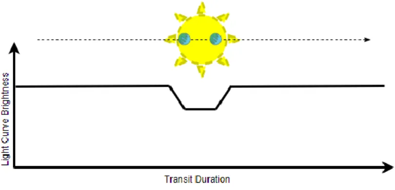
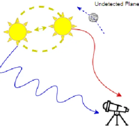
The Kepler mission monitored and cataloged data to support classic exoplanet identification techniques of transit time, radial velocity, microlensing, and direct imaging. Radial velocity measures the shift of a star as from the gravitational pull of its orbiting planets. The measurement of radial velocity is correlated to the mass and the orbital period of a planet. Increases in mass and orbital speed result in increases in radial velocity [2]. Microlensing is an indirect method of planet detection [2]. It measures the bending of light as energy from a star passes a planet [2]. Microlensing offers the ability to detect the smallest and most distant planets. Direct imaging is one of the oldest techniques used to identify exoplanets. This method involves using high-powered terrestrial and extra-terrestrial telescopes to capture detailed pictures of star fields. The pictures are then examined by man and machine to determine if planets exist. While this method is good for detecting stars, direct imaging has proven to be inadequate for exoplanet identification [2]. The descriptions of radial velocity, microlensing, and direct imaging are intentionally brief as this work focuses primarily on transit time and cumulative data.
Fig. 1. Transit time10.
8 https://exoplanetarchive.ipac.caltech.edu/index.html
9 https://www.vox.com/science-and-health/2018/11/1/18049028/kepler-space-telescope-retire-nasa 10 As a planet crosses between a star and the field of view of the observation tool, the light curve is altered.
The transiting planet absorbs, reflects, or redirects a portion of the energy detected by the observer. The speed of transit and magnitude of the light curve change provide several insights into the object
Fig. 2. Radial Velocity11.
Transit time was briefly discussed in the previous section and was an area of concentration for this study. Planetary transits can yield information which can lead to an estimate of the
object of interest’s size, speed of orbit, period of orbit, mass, and density of its star [2]. Amazingly, a transit can also provide clues to an object of interest’s atmospheric composition
as different elements absorb and reflect light differently [2].
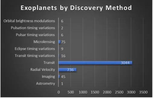
Fig. 3 illustrates how dramatically the Kepler mission altered the science of exoplanet discovery. Its revolutionary mix of exoplanet identification techniques has ushered in a new era
of rapid exoplanet detection. Kepler’s transit data has become the leading source of data and
method for identifying exoplanets. Traditional direct imaging and radial velocity techniques are biased towards the detection of large exoplanets. In contrast, Kepler’s transit time data
allows for the detection of smaller Earth-sized exoplanets—opening a whole new window of planets to be discovered [4].
A critical element to identifying a potentially habitable exoplanet is determining if the object
of interest is in a solar system’s “Habitable Zone”. This zone is based on the fundamental
requirements for life known today—primarily the possibility of liquid water on a planet’s
surface [5]. Using our solar system as an example, we can conclude that Earth sits within a habitable zone. Earth has an abundance of liquid water and life. Planets closer to the sun like Venus, are too hot to support life as we know it; while planets further out like Mars and beyond thought are too cold. Using a combination of transit time and other measurements collected
by Kepler, it is possible to determine approximate a star’s habitable zone as well as the type and
distance from the star any planets might be. Together these parameters allow scientist to estimate the probability that a given planet might be able to support life.
crossing the star. Detecting light curve variations caused by transiting planets has become one of the more reliable methods of detecting exoplanets. https://www.jpl.nasa.gov/edu/teach/activity/exploring-exoplanets-with-kepler/
11The gravitational pull of an orbiting planet tugs on its star. This causes a “Doppler Shift” in the star’s spectra. As seen above, shifts between the blue and red ends of the star’s spectra can be observed as a
Fig. 3. The horizontal bar chart shows total confirmed exoplanets by discovery method. The time period for the graph is 1989 to 2018. The planet transit method is, by far, the most influential technique used to discover exoplanets. Radial velocity is the next highest method of discovery12.
Another exoplanet dataset used for classifying candidate objects of interest is the Cumulative Kepler Object of Interest (KOI) table13. The KOI table contains aggregate level data describing unique object of interest identifiers, exoplanet archive attributes, project disposition columns, summarized transit properties, threshold-crossing events, stellar parameters, and pixel-based KOI vetting statistics14; and considering the subject matter and vast distances of which the data was collected, the data quality of this table is good given the subject matter.
3 Methods
3.1 Machine Learning
Machine learning is a subset of the greater field of artificial intelligence. Machine learning combines computer programming and statistical theory to construct models to make inferences based on data. These inferences can be a pattern, description, or prediction based on past data [6]. For exoplanet identification, this study focuses on utilizing machine learning for the classification of objects-of-interest as exoplanets or “false positives”. Machine learning is not tool specific; models are available in a variety of methodologies, software packages, and tools.
12 https://exoplanetarchive.ipac.caltech.edu/docs/counts_detail.html 13
https://exoplanetarchive.ipac.caltech.edu/cgi-bin/TblView/nph-tblView?app=ExoTbls&config=cumulative
All computer programming for classifying objects-of-interest in this study was done using Python.
3.1.1 Python and Machine Learning
Python is an open-source object-oriented language developed by Guido Van Rossum. It was developed with the goals of producing highly readable code which is relatively easy to learn yet capable of solving complex problems15. Python is one of the most popular and widely used programming languages by data scientists globally. In July of 2018, Information Week listed Python as one of the top-five languages for data science16. Kaggle’s “State of Data Science
and Machine Learning” study in 2017 lists Python as the most commonly used language in data
science17. In addition to the reasons listed above, several statistical and machine learning packages are compatible with Python; allowing the functionality to be customized to fit the needs of a variety of data science use cases. Virtually all commonly used—supervised and unsupervised—machine learning algorithms are available in Python through a third-party package.
3.1.2 Scaling Data
While not always required for machine learning models, scaling data is often used to ensure all data features exist on a comparable scale [7]. For example, the cumulative KOI data contains a column for equilibrium temperature in degrees Kelvin. The minimum recorded value in the data set for equilibrium temperature is 25°. The maximum recorded value is over 14,000°K. Stellar surface gravity is another column available in the KOI data. It has a minimum recorded value of 0.047 and a maximum of 5.364. Such a drastic difference in scale could falsely influence the classification of exoplanets. Scaling data converts all features to the same scale. For instance, a scale of zero to one is often used to define the minimum and maximum values of features after data is scaled. Functions available in Python libraries automate this task [7]. 3.1.3 Cross-Validation
The intent in developing machine learning models for prediction is to apply the model to unseen data [7] [8]. A common concern for a newly created machine learning model is overfitting that model to the data used to train it. Overfitting essentially biases a model to make predictions based on the unique nuances of the training data that are not present in the universe of data as a whole [9]. The resulting predictions made when applying the overfit model to new data is sub-optimal predictions. One method to combat overfitting is to use cross-validation. During cross-validation of large data sets, the data set is divided into subsets based on specified parameters. The model is trained on the subset of the data set and then scored against the portion of the data set which has not used for training [8]. This effectively simulates exposing
15 https://www.python.org/about/
16
https://www.informationweek.com/big-data/ai-machine-learning/5-top-languages-for-machine-learning-data-science/d/d-id/1332311?page_number=6
the model to fresh data outside the training dataset. Cross-validation is a critical step in the creation and validation of machine learning models.
3.1.4 Feature Elimination
Feature elimination is another important step in building a machine learning model which can be generalized and applied to new data sets. Several machine learning models do not perform feature elimination on their own [10]. Feature elimination should be utilized when there are many features or columns in the data set. For example, the Cumulative KOI data set contains over eighty features. Some features are highly important to classifying objects of interest; other features have limited predictive ability. It is necessary to identify and remove the features with limited predictive ability to create a generalized model which can be applied to new datasets. There are several manual, statistical and programmatical techniques which can assist with feature elimination.
3.1.5 Classification
There are three primary categories of machine learning solutions: regression, clustering, and classification. Classification is a form of supervised machine learning where observations are assigned a known class value based upon their explanatory variables. Classification values can be binary or multi-class. This study focuses on a binary classification of objects of interest
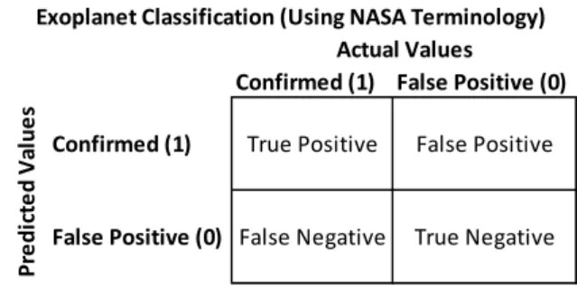
as “FALSE POSITIVE” or “CONFIRMED” exoplanets. The classification of “FALSE POSITIVE” is used by NASA to indicate the satellite incorrectly tracked an object of interest.
The meaning of the term in machine learning classification terms is a bit different.
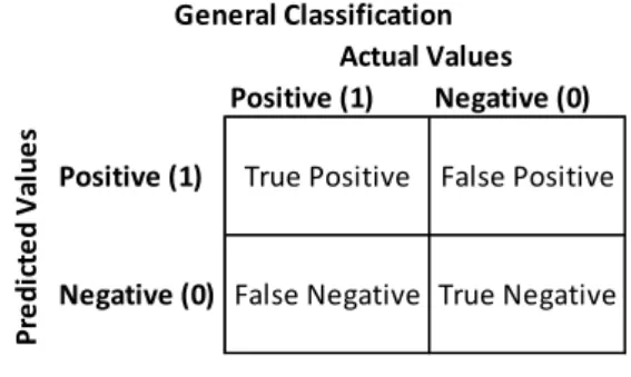
A “False Positive” in classification occurs when an observation is predicted to be positive
when it is actually negative. As shown in Fig. 5, the NASA exoplanet disposition of
“FALSE POSITIVE” is simply a synonym for “Negative” in
Fig. 4.
Fig. 4. Picture showing the meaning of True Positive, False Positive, False Negative and True Negative in binary classification.
Positive (1) Negative (0)
Positive (1) True Positive False Positive
Negative (0) False Negative True Negative
Actual Values Pr e d ic te d V al u e s General Classification
Fig. 5. Binary classification of candidate exoplanets using NASA terminology.
Classification algorithms can be evaluated using a variety of metrics. Three common metrics used are accuracy, precision, and recall. For all three metrics, a higher score is better. Accuracy is a simple score which measures how many correct predictions were made. Precision helps score models which make few incorrect positive classifications. Recall helps assess how well models correctly classify negative classifications. The equations for all three metrics are shown below:
Accuracy = (True Positives + True Negatives) ÷ Total Predictions . (1) Precision = True Positives ÷ (True Positives + False Positives) . (2) Recall = True Positives ÷ (True Positives + False Negatives) . (3)
3.1.6 Support Vector Machine (SVM) / Support Vector Classifier (SVC)
Support Vector Machines are non-parametric algorithms which seek to identify a hyperplane that maximizes the distance between the hyperplane and points in opposing classes of the dataset [11]. Fig. 6, shown below, shows a simple hyperplane example. The different color and shape dots represent different classes in the data. The dashed lines represent the support vectors which define the maximum margin of the hyperplane.
Fig. 6. SVM Hyperplane Example
Confirmed (1) False Positive (0)
Confirmed (1) True Positive False Positive
False Positive (0) False Negative True Negative
Actual Values Pr e d ic te d V al u e s
Fig.6 is a simplistic example for illustration purposes. As with any classification algorithm,
misclassifications can and will occur. The “C” parameter can be adjusted to define how
important misclassifications to the algorithm. A large “C” minimizes misclassifications with
a narrow margin. A small “C” value creates a broader margin and allows for more misclassifications [11].
3.1.7 K-Nearest Neighbors (KNN) Classifier
K-Nearest Neighbors for classification assigns a label to unclassified observations based on the
“k” nearest classified observations in space. The “k” parameter value directs the KNN
classification algorithm to label an unclassified observation based on the classification of the
“k” observations which are most like the unclassified observation. Choosing the appropriate
value for “k” is a combination of art and science. The optimum value of “k” can be determined
using parameter selection techniques and cross-validation. However, expert intuition and domain knowledge are also helpful in determining the most practical value for “k”. KNN models are proven to be useful in scenarios where the dataset contains a limited number of dimensions with a large number of observations [12].
3.1.8 Random Forest Classifier
Random Forest classification consists of an ensemble of decision trees. Random forests utilize bagging and randomized feature selection to build the ensemble of decision trees [13]. Bootstrap aggregations, bagging, set a strategy of sampling X observations from the dataset with replacement from the X observations [13]. The bagging strategy results in only a portion of the available dataset being utilized in any single decision tree in the ensemble. Like cross-validation, this helps to generalize the model. Random feature selection works exactly as it sounds. A subset of the features from the dataset is randomly selected to construct individual decision trees in the ensemble [13]. This helps to generalize the model as well. The effects of correlation and overfitting can be reduced by utilizing random feature selection. The ultimate classification is obtained by combining the results of each tree in the ensemble to reach a decision [13]. Random Forest models are robust to high dimensional data and generally do not require data to be scaled to function correctly.
3.2 Pipeline for Machine Learning Models
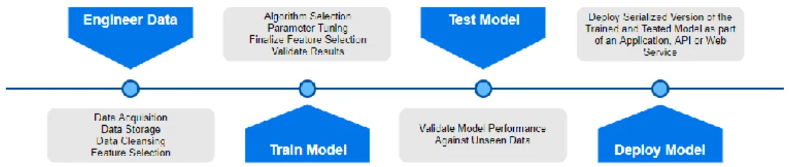
A machine learning pipeline outlines the steps taken to turn a candidate data set into a functioning machine learning model. As shown in Fig. 7, source data sets are staged for data engineering. The output of data engineering is used to train a machine learning model. This is an iterative step as discoveries made during model training can influence data engineering steps. Once a suitable trained model is available, the model is tested against unseen data to assess the suitability for deployment to a production environment. A trained and tested model can then be serialized and deployed as a production model which can be accessed in a variety
of ways. The model can be exposed to users and systems via API, or executed as part of a larger process.
Fig. 7. Machine Learning Data Pipeline. The machine learning data pipeline is a visual depiction of the steps taken to produce the Random Forest Classifier developed in this study.
3.3 Application Programming Interfaces (APIs)
APIs are commonly developed to provide a method of interoperability between different systems, models and code bases. APIs provide an interface between developers and the systems with which the developers are looking to access [14]. For example, a machine learning model created by a data scientist in python may not be useful to a production support technician proficient in Java. Instead of rewriting the model in Java, the model can be exposed via API to the production support technician. The API is constructed using specific arguments defined by the API developer. The correct use of the API arguments allows the user of the API to interact with the target system.
3.4 Cloud Computing
Cloud computing represents the democratization of infrastructure. Cloud computing vendors offer products on a service basis. Instead of building out and maintaining dedicated server farms, companies of all sizes can outsource this function to a cloud vendor. Cloud Computing modes of service typically include Infrastructure as a Service (Iaas), Platform as a Service (PaaS) and Software as a Service (SaaS) [15]. No two cloud computing vendors are the same. However, cloud computing relies upon some ubiquitous concepts: virtualization, service-oriented architecture and web services.
This study leveraged cloud computing services of the Google Cloud Platform and
Microsoft’s Azure Cloud. Within the Google Cloud Platform, IaaS was utilized in the form of a Linux Ubuntu server. The IaaS server was used to create the machine learning model and host a simple API as a web service. PaaS products such as a prebuilt data science virtual machine and Azure Container Services were employed in Azure to host a containerized web service.
4 Analysis
4.1 Machine Learning Model Selection
The KOI table is a data source ripe for the application of machine learning. For this paper, KNN, SVM, and Random Forest models were created, cross-validated, and inspected for accuracy, recall, and precision to arrive at the superior model for object-of-interest classification. The end predictions from each model were also manually inspected to determine if the results met rough expectations for the number of observations classified as exoplanets. The Random Forest model was selected for the classification of Cumulative KOI observations. Fig. 8 shows the rationale for proceeding with Random Forest classification. While all three algorithms trained well, SVM did not produce expected prediction results in terms of the proportion of observations classified as exoplanets. A variety of feature and parameter combinations were attempted with SVM without improvement in the results. While feature reduction could mitigate a large number of dimensions in this data, KNN, SVM, and random forest methodologies are naturally robust to high dimensionality. An important decision point for the team was “explainable machine learning”. Random Forest produces scaled feature importance values which clearly show the most and least important features in classifying data. KNN and SVM are somewhat of a black box in that feature importance is not calculated since the distance between points (KNN) and hyperplane separation (SVM) define the optimal model.
Fig. 8. This table shows the inputs to deciding to proceed with Random Forest Classification of cumulative KOI observations. All points are debatable and are not intended to say any model is unsuitable for this task. Instead, the table provides insight into
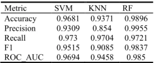
Table 1. Training metrics or SVM, KNN and Random Forest Models.
Metric SVM KNN RF Accuracy 0.9681 0.9371 0.9896 Precision 0.9309 0.854 0.9955 Recall 0.973 0.9704 0.9721 F1 0.9515 0.9085 0.9837 ROC_AUC 0.9694 0.9458 0.985
Table 1 shows the three classification models all performed well using the training data set. However, the Random Forest produced generally superior numbers. The balanced F1 score favors the Random Forest classifier. Metrics in the high nineties raise the risk of overfitting the dataset. However, stratified shuffle split validation, feature reduction,
cross-validated parameter selection, and manual parameter tuning where all employed to guard against over-fitting. Additionally, the bagging and random feature selection native to Random Forest Classifiers provide additional safeguards against overfitting. The Random Forest Classification model was utilized for classification of the Cumulative KOI data.
4.2 Data Engineering
Data preparation covers all steps and procedures taken to prepare the Cumulative KOI data for input into machine learning models. Machine learning algorithms often have strict data requirements. For example, most scikit-learn python classifier algorithms are not robust to missing values, and some models produce superior results if all data attributes are on a similar scale.
4.2.1 Load and Cleanse Data
The Cumulative Kepler Object of Interest table is updated relatively infrequently. The data in this table is relatively clean. However, there were some areas which required attention before building the Random Forest classification model. First, we begin by examining the data manually and programmatically to assess the availability of values within features. Next, features with no or limited predictive ability are dropped. This includes unique identifiers, raw text comment fields and database constructs such as row identification numbers. Third, there are several columns which inject leakage into the model. Leakage is a term meant to describe any feature which provides enough information to know what should be the predicted outcome.
For instance, if the “kepler_name” attribute is populated, this indicates scientists have confirmed a Kepler Object of Interest to be an exoplanet. Fourth, there are two columns which are essentially the same. “koi_time0bk” adjusts “koi_time0” by a constant offset18. This results in a 100% correlation between the two columns. Therefore, “koi_time0bk” is removed from
the dataset. Finally, the level of uniqueness of the remaining columns is checked to see if there are any remaining features which may have no or low uniqueness or variance. Features with no or low variance have limited benefit to the predictive model. If all values for a feature in a dataset are the same, a model could not use that feature to differentiate between observations.
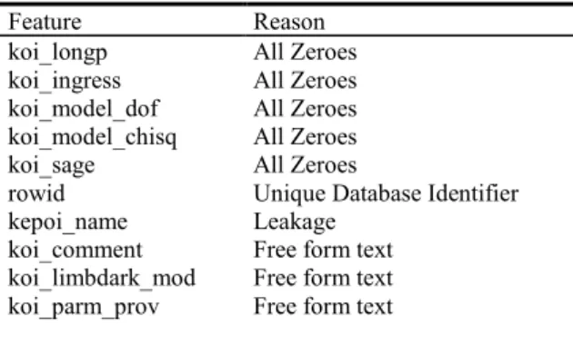
Table 2. List of all columns dropped from the analysis data set during initial data cleansing steps.
Feature Reason
koi_longp All Zeroes
koi_ingress All Zeroes
koi_model_dof All Zeroes
koi_model_chisq All Zeroes
koi_sage All Zeroes
rowid Unique Database Identifier
kepoi_name Leakage
koi_comment Free form text
koi_limbdark_mod Free form text
koi_parm_prov Free form text
Feature Reason
koi_trans_mod Free form text
koi_datalink_dvr Free form text koi_datalink_dvs Free form text
kepid Unique identifier
koi_pdisposition Leakage
kepler_name Leakage
koi_score Leakage
koi_time0bk Duplicate
koi_tce_delivname Free form text
koi_sparprov Free form text
koi_vet_stat Zero variance
koi_vet_date Zero variance
koi_disp_prov Zero variance
koi_ldm_coeff3 Zero variance
koi_ldm_coeff4 Zero variance
4.2.2 Missing Values
There are known causes of missing values due to data, software and hardware issues encountered during the Kepler mission [16]. This data is missing at random (MSAR), monotonic19, and primarily continuous data. The work of Morton describes these issues in detail. In most cases, NASA scientists discard observations with data issues [16]. However, this research sought to preserve these observations through different imputation methods. Two different strategies were explored for the cumulative KOI dataset: zero filling and K-Nearest Neighbors (KNN) imputation. Filling missing values with zeros should be used with caution. This is typically used when missing values are an accurate representation of the data. This is not the case for this dataset.
KNN imputation is a single imputation technique which seeks to fill missing data within an
observation based on the mean value of that observation’s K nearest neighbors [17]. The K parameter is best selected using cross-validation and model scoring. A common suggestion for the K parameter to use the square root of the number of observations in the dataset [17]. This study used eighty-three (√9564) for the K parameter. Two datasets, zero-filled and KNN imputed, exist after this step. A multiple imputation technique was not tested. A key benefit of multiple imputation is the imputed values determined by multiple imputation preserve the otherwise natural variance of the dataset [18]. However, if a sufficiently large K parameter is selected, KNN imputation can provide a close approximation of the natural variance of the dataset using values which actually occur in the dataset [19]. Additionally, the monotonic pattern of missingness is well suited for predictive methods of imputation20. By using KNN imputation, approximately 930 observations can be retained for input into the Random Forest Classifier. 19 https://support.sas.com/documentation/cdl/en/statug/63033/HTML/default/viewer.htm#statug_mi_sect 017.htm 20 https://support.sas.com/documentation/cdl/en/statug/63033/HTML/default/viewer.htm#statug_mi_sect 018.htm
4.2.3 Correlation
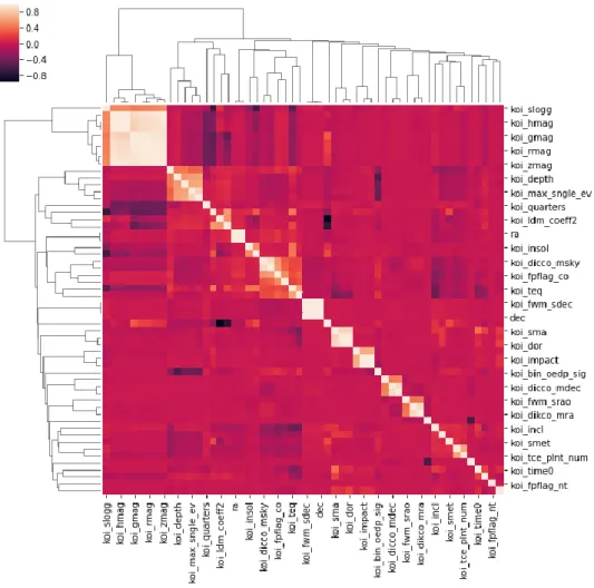
Random Forest models are naturally resistant to multicollinearity in datasets due to bagging and random feature selection2122. Fig. 9 is a hierarchical correlation plot showing areas of highly correlated data in the data after data cleansing. Fig. 9 shows multicollinearity is largely a non-issue in the cumulative KOI dataset. However, the upper left-hand corner of the correlation plot shows a cluster of eight highly correlated features. If necessary, several of these features could be removed to reduce processing time for the Random Forest Classifier.
Fig. 9. Correlation Plot after feature reduction.
21
https://towardsdatascience.com/seeing-the-random-forest-from-the-decision-trees-an-intuitive-explanation-of-random-forest-beaa2d6a0d80
4.2.4 Bias
Bias may be a cause for concern in this dataset. One method used by the Kepler team is to direct the satellite to hunt for objects of interest in areas where other planets have already been found (1). Of course, this strategy makes logical sense given the obvious enormity of scanning the universe. However, this course of action could have unintended impacts on machine
learning models. For example, the “koi_count” column indicates the number of candidate
planets identified in a system23. Initial testing with Random Forest Classifiers identified the
“koi_count” column as the most important feature in the dataset. Therefore, an object of interest with similar features as a confirmed planet could be classified as a “false positive”
simply due to there not being a candidate planet being detected in its system. Thus, the
“koi_count” column was removed from the dataset ultimately input into the Random Forest
Classifier.
Additionally, an article from Time magazine in December 2011 stated the team expected 90% of the batch of objects of interest identified at that time to end up being classified as exoplanets. Over time, the percentage of objects of interest determined to be planets is closer to approximately 35% with the percentage increasing per batch over time. To be clear, this
isn’t a statement on ethics. The Kepler team is chartered to discover exoplanets for input into scientific research. As such, casting a wide net to produce realistic observations for scientists to study does make sense. However, it provides the data scientist hints on the metric to use to train and evaluate machine learning models. It may be wise to train classification models to optimize based on recall to penalize false positives.
4.3 Model Training
4.3.1 Create Train and Test Datasets
Creation of train and test datasets is a common practice in developing a machine learning model. The training dataset for a classification problem contains labels showing the classification of known observations. This allows a machine learning algorithm to “learn”, or be trained, based on past data. The test data set is used to validate the trained model. The test data set for a classification problem is not labeled. The machine learning model has to classify the observation based on the rules and parameters defined during model training.
Fortunately, the Cumulative KOI table has each observation labeled with a disposition of
“FALSE POSITIVE”, “CONFIRMED”, OR “CANDIDATE” in the “koi_disposition”
column24. This enables the creation of a training data set with observations with a disposition
of “FALSE POSITIVE” OR “CONFIRMED”. “FALSE POSITIVE” is used to describe all
objects of interest tracked by Kepler which were determined not to be exoplanets.
“CONFIRMED” describes objects of interest which have been confirmed to be exoplanets. “CANDIDATES” have not yet been formally classified25. The “CANDIDATE” observations create the test dataset used to make the final classification of exoplanet or not. For the train
23 https://exoplanetarchive.ipac.caltech.edu/docs/API_kepcandidate_columns.html 24
https://exoplanetarchive.ipac.caltech.edu/cgi-bin/TblView/nph-tblView?app=ExoTbls&config=cumulative
dataset, the disposition is encoded to a binary numeric column as required by the SVM classifier
in Python (0 = “FALSE POSITIVE”, 1 = “CONFIRMED”)26. This variable is then split into its own dataframe and dropped from the primary dataset. The disposition dataframe is the response variable for the SVM classifier.
4.3.2 Cross-Validation and Parameter Selection
Interestingly, approximately two-thirds of the observations in the training data set are not
exoplanets (“FALSE POSITIVES”). With the relatively high differences between objects of interest which are and are not exoplanets, stratified shuffle-split cross-validation was selected to build the cross-validation objects with ten folds. Stratified cross-validation is useful when there is a relatively large imbalance in the number of positives and negatives in a training data set. Stratified cross validation creates folds which seek to preserve the percentage of classifications present in the source dataset27.
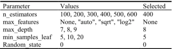
Random Forest parameter selection was facilitated using sklearn’s “GridSearchCV”
function28. Using “GridSearchCV” a grid of parameter options can be created and passed to the function. “GridSearchCV” uses the parameter grid, a support vector machine model object and the cross-validation object described above to iterate through each discrete combination of parameters using accuracy as the guide to select the optimal parameter combination29. This handy function allows the developer to bypass manual examination of various models or creating a custom script to score parameter combinations. The components of the parameter grid and result are shown below:
Table 3. GridSearchCV Parameters30 . The “Selected” column also shows the optimal parameter
combination as identified by GridSearchCV.
Parameter Values Selected
n_estimators 100, 200, 300, 400, 500, 600 400 max_features None, "auto", "sqrt", "log2" None
max_depth 7, 8, 9 8
min_samples_leaf 5, 10, 20 5
Random_state 0 0
4.4 Feature Importance
As previously mentioned, explainable feature importance is a key differentiator of Random Forest when compared to K-Nearest Neighbors (KNN) and Support Vector Machine (SVM) classification. Feature importance was generated for each field across ten-fold stratified shuffle-split cross-validation testing, as well as against the entire training data set. Fig. 10
26 http://scikit-learn.org/stable/modules/generated/sklearn.svm.SVC.html 27 http://scikit-learn.org/stable/modules/cross_validation.html#cross-validation-iterators-with-stratification-based-on-class-labels 28 http://scikit-learn.org/stable/modules/generated/sklearn.model_selection.GridSearchCV.html 29 http://scikit-learn.org/stable/modules/grid_search.html 30 https://scikit-learn.org/stable/modules/generated/sklearn.ensemble.RandomForestClassifier.html
shows overall feature importance as identified by the Random Forest classifier. Table 4 contains a brief categorization of all features plotted in Fig. 10.
Fig. 10. Overall Feature Importance.
Table 4. Top eight cumulative KOI features as determined by the Random Forest Classifier31. Full
scientific descriptions of each feature in table four can be found following the hypertext link in footnote 31.
Feature Feature Category
koi_prad Planet Radius
koi_dicco_msky Angular Offset
koi_fpflag_nt Transit
koi_fpflag_ss Transit
koi_fpflag_ec Similarity to confirmed exoplanets koi_fpflag_co Transit and presence in a solar system
ENC_LS+MCMC One hot encoded column from “koi_fittype”. Similarity to confirmed exoplanets.
koi_dikco_msky Angular Offset
To summarize the meaning of the top-ten features, the object of interest’s: size; transit data, angular offset, similarity to other confirmed planets, and presence in a solar system appear to have the greatest impact object of interest classification. The plots shown in Fig. 11 below show objects of interest which have been classified as planets were typically smaller in radius (similar to the size of earth); had a shorter transit duration; and had an angle of offset close to zero.
Fig. 11. Distribution and scatterplots illustrate the relationship between important feature concepts and exoplanet classification. Radius, transit duration, and angular offset overlaid distribution plots show frequency and levels of classified objects of interest.
5 Results
5.1 Random Forest Classifier Results
The accuracy, precision, recall, F1, and ROC AUC scores are presented in Table 1. As discussed, the Random Forest performed well against the training dataset; however, measures were taken to prevent overfitting and bias in the data, those concerns persist as the Random Forest model predicted approximately 49% of the candidate observations which have a 90% or greater chance of being an exoplanet. 39%, or 968 candidate observations, have a greater than 95% chance of being an exoplanet. Given the historical classification rate of exoplanets, a greater than 95% chance of being an exoplanet is likely to be an appropriate cutoff for serious consideration of being an exoplanet. That said, findings from past planets have influenced the classification of newer objects-of-interest. For example, objects-of-interest with a radius of roughly two times the size of Jupiter or greater are treated as noise and are now automatically classified as false positives [20] [21]. This results in a maximum radius in the test dataset of 109,061 compared to 200,346 in the training data. Similarly, the maximum transit duration in the test dataset is 44.35 versus 138.54 in the training data. Therefore, the random forest
classifier may not be overfitting at all; it may be simply performing as intended against evolving exoplanet detection statistics. Comparing Fig. 11 to Fig. 12 below suggests the random forest classification of the test dataset followed the boundaries set during model training. Though the overall maximum distribution of key features changed, the algorithm continued to classify objects-of-interest with a smaller radius, shorter transit duration, and low angle of offset as exoplanets.
Fig. 12. Distribution and scatterplots generated based on the classification of the test dataset. Comparison to the scales of objects classified as exoplanets in Fig. 11 shows similar results were obtained.
As previously mentioned, this machine learning model provides a verified, automated method of classifying cumulative Kepler objects of interest as planets. When correctly used, this algorithm offers an avenue to expedite the classification of objects-of-interest based on the characteristics available in the KOI table.
5.2 Model Deployment
Fig. 13. The comprehensive process for creating and deploying the random forest cumulative Kepler object of interest classifier.
Fig. 13 depicts the overall process and tools used to train and deploy the random forest classifier model described above for broader use. The overall strategy used on this project was to train locally then deploy globally in the cloud. Though training was performed on a virtual machine (VM) in the Google Cloud Platform, this is considered local training as the model was built and tested on a single private VM. The first option explored for deployment of the random forest model was conducted using a Flask API on the same Google Cloud VM used for training. A simple python application loaded the serialized version of the random forest classifier and instantiated a Flask endpoint capable of accepting a JSON formatted classification request using. JSON (JavaScript Object Notation) is a readable data structure typically used to transmit information between servers and web applications32. A sample JSON document is included in Appendix D for reference. The Flask API is a simple, low-cost method for exposing machine learning models for broad use—though there are some questions about the scalability of Flask APIs for widespread use.
To improve scalability, the same serialized random forest classifier created in the Google
Compute engine was ported to Microsoft’s Azure Cloud environment. Once the model was
loaded to the Azure Cloud, it is registered and deployed using Azure Container Instances (ACI). Two code-based steps are required to register the machine learning model. First, a Python program which generates a container environment file is created. The container environment file contains the python version and libraries required to operate. Second, a Python-based scoring file is created to parse the JSON document and classify the observation. ACI offers a quick, scalable method of creating and deploying a machine learning model as a web service33. Furthermore, the container-based platform allows for seamless future modifications and upgrades to the random forest classifier. A new container with an updated classifier can be deployed alongside an existing classifier. Once the new container to ready for use, the old container can be retired, and requests are routed to the new container. The ACI accepts the same JSON document shown in Appendix D and returns the probability of the observation being an exoplanet. As of this writing, the returned probability contains two values. The first in
32 https://developers.squarespace.com/what-is-json
the probability of the observation not being an exoplanet. The second is the probability of the observation being an exoplanet.
6 Ethics in Exoplanet Identification
Ethics in science are the moral principles which set the boundaries for research. Many studies and codes have been created to define ethical conduct in medicine, government, and corporate research. Practiced ethically, science can build trust between scientific disciplines and the general public. It is easy to understand the importance of ethical research when human life is involved. However, the implications of ethics are subtler when applied to astronomy.
As a science, astronomy strives to build a body of knowledge to increase humanities understanding of the universe34. However, ethics in astronomy is critical from educational, environmental, and financial perspectives. Astronomical research creates the body of knowledge by which future astronomers are trained. Astronomers have a moral duty to produce accurate and unbiased research by which future scientists are educated [22].
Unethical research could have a “butterfly effect” which could negatively impact scientific
training for years. As seen with this study, the Kepler mission was an expensive endeavor requiring significant government and private funding [2]. Falsifying data and inflating the
quantity and quality of exoplanets could jeopardize future missions. NASA’s Exoplanet
Program has a long-term strategy with multiple missions scheduled over decades. Funding for these missions could be jeopardized if unethical work is used to justify these missions. Astronomy is applied to a wide range of projects. Some of these projects could be critical to the long-term health of the planet and its inhabitants35. For example, the study of climate change requires astronomy for surveillance and measurement of the changing environment. Ethical astronomy builds public trust in the science and can aid in increasing public awareness and education. Ethical astronomy builds trust in those who depend upon the science for professional, social, and environmental health. Ethical practices for astronomy must be curated and applied to studies to remain a credible science.
This study has attempted to apply ethical statistical and machine learning principles. Feature reduction, parameter selection, bias assessments, and model selection in this study all
offer opportunities to review the ethical quality of the team’s decision making. These activities present avenues where ethical concerns could arise. The team addressed the potential pitfalls by utilizing standardized methods (Python libraries and proven statistical methods), explainable machine learning, and overall transparency. Applying standardized methods, explainable machine learning, and transparent research is required to reach a reproducible conclusion. The detailed documentation of this study allows for independent peer review by anyone looking to build on the results of this work. The work can be reviewed by experts in Astronomy and machine learning to validate the efficacy of this research.
A code of ethics for machine learning and data science does not currently exist. Ethical applications of machine learning are critical to creating professional and public trust in this discipline. Machine learning is used in a wide array of use cases around the world. Features, parameters, and measurements should not be altered for the sole purpose of reaching the desired conclusion. As with astronomy, machine learning is a critical tool to assist with solving
34 https://aas.org/eth
humanities most pressing issues. The results of machine learning must be produced with the utmost adherence to ethical research for decision makers to believe in machine learning conclusions and base policy decisions based on machine learning results.
7 Conclusions
The primary objectives of this study were to create a machine learning model to automate the classification of Kepler cumulative object of interest data and deploy that model to the outside world. To achieve this goal, a comprehensive machine learning pipeline was created to engineer the data, train, and test models. This process attempted to produce a set of candidate features after accounting for missingness, statistical inconsistencies, correlations, and bias. These candidate features were used to train K-Nearest Neighbor (KNN), Support Vector Machine (SVM) and Random Forest classifiers. Based on model performance and explainable feature importance, the Random Forest classifier was chosen as the primary model for testing and deployment. The Random Forest classifier identified radius, transit characteristics, and angle of offset as features with the highest importance for classifying objects-of-interest. Objects-of-interest with a radius between Mars and Neptune, a transit light curves similar to other confirmed planets, and an angle of offset less than five are most likely to be classified as exoplanets. Use of the random forest model can automate and supplement the routine work needed vet Kepler objects of interest by highly skilled scientists and astrophysicists.
The production deployment of a machine learning model represents the culmination of many data science projects. Basic knowledge in this area is an important ingredient in any data scientist’s tool kit. In this study, two methods of deployment were examined. First, Flask was utilized by a python application to create an API to answer classification requests with a probability of the observation being an exoplanet. This method offers a low-cost, reliable method to deploy a production machine learning model. However, there are questions about the ability of a Flask API to meet increased demands. Therefore, a second, more robust, and scalable technology set in the Microsoft Azure Cloud was implemented to achieve the same result as the Flask API but with improved scalability. The random forest exoplanet classifier was registered in the Azure Cloud and deployed as an Azure Container Instance (ACI). The ACI accepts and responds to classification requests as well, but it offers more robust capabilities to meet increased demands. The nature of container technology also offers the advantage of performing seamless model updates with little to no customer impact.
Finally, a concerted effort was made to support the concept of ethical, reproducible research. All steps and methods documented in this study can be recreated to verify the results. Teams with higher levels of domain expertise may be able to leverage components of this work to further their own scientific efforts. As one of humanities oldest scientific disciplines, astronomy continues to fuel scientific discoveries. In the near future, the science of astronomy may be used to solve some of the more pressing problems faced by our planet. An honest examination of exoplanets and their formation may help unlock the keys to improving life earth.
References
1. Shallue, Christopher J and Vanderburg, Andrew. Identifying Exoplanets with Deeo Learning: A Five Planet Resonant Chain. Harvard-Smithsonian Center for Astrophysics. [Online] 12 16, 2011. https://www.cfa.harvard.edu/~avanderb/kepler90i.pdf.
2. Exoplanet Science Strategy. Washington, DC : National Academies of Sciences, 2018. 3. Borucki, William J., et al. Kepler Planet-Detection Mission: Introduction and First Results.
Science. 2 19, 2010, pp. 977-980.
4. Clery, Daniel. Kepler telescope catalogs hundreds of new alien worlds, some potentially
habitable. www.sciencemag.org. [Online] 6 19, 2017.
http://www.sciencemag.org.proxy.libraries.smu.edu/news/2017/06/kepler-telescope-catalogs-hundreds-new-alien-worlds-some-potentially-habitable.
5. Kane, Stephen. Habitable Zone Dependence on Stellar Parameter Uncertainties. 11, February 20, 2014, The Astrophysical Journal, Vol. 782, pp. 111-119.
6. Alpaydin, Ethern. Introduction to Machine Learning. Third. Cambridge : The MIT Press, 2014.
7. Raschka, Sebastian. Python Machine Learning. Birmingham : PACKT, 2015.
8. Ramsey, Fred and Schafer, Daniel. The Statistical Sleuth. Third. Boston : Brooks/Cole, 2013.
9. Dietterich, Tom. Overfitting and Undercomputing in Machine Learning. ACM Computing Surveys. September 3, 1995, Vol. 27.
10. Hastie, Trevor, Tibsharani, Robert and Friedman, Jerome. The Elements of Statistical Learning. Second. New York : Springer, 2008.
11. Leskovec, Jure, Rajarman, Anand and Ullman, Jeffrey. Mining of Massive Datasets. New York : Cambridge University Press, 2014.
12. Kramer, Oliver. K-Nearest Neighbors. Dimensionality Reduction with Unsupervised Nearest Neighbors. Berlin : Springer, 2013, pp. 12-23.
13. Gray, Katherine, et al. Amsterdam. Random forest-based similarity measures for multi-modal classification of Alzheimer's disease. Elsevier, 2013, NeuroImage, Vol. 65, pp. 167-175.
14. Myers, Brad and Stylos, Jeffrey. Improving API Usability. Communications of the ACM. 2016, Vol. 59, 6, pp. 62-69.
15. Al-Masah, Ahmed and Al-Sharfi, Ali. Benefits of Cloud Computing for Network Infrastructure Monitoring Service. International Journal of Advances in Engineering and Technology. January 2013, Vol. 5, 2, pp. 46-51.
16. Morton, Timothy, et al. False Positive Probabilities for All Kepler Objects of Interest: 1284 Newly Validated Planets and 428 Likely False Positives. s.l. : The American Astronomical Society, May 10, 2016, The Astrophysical Journal, Vol. 822, pp. 86-100.
17. Huanga, Jianglin, et al. Cross-validation based K nearest neighbor imputation for software quality datasets: An empirical study. July 13, 2017, The Journal of Systems and Software, pp. 226-252.
18. Sterne, Jonathon, et al. Multiple imputation for missing data in epidemiological and clinical research: potential and pitfall. 7713, s.l. : British Medical Journal, July 18, 2009, Vol. 339, pp. 157-160.
19. Beretta, Lornenzo. Nearest Neighbor Imputation Algorithms: A Critical Evaluation. s.l. : BioMed Central, July 25, 2016.
20. Livingston, John H., et al. 44 Validated Planets from K2 Campaign 10. The Astronomical Journal. 2018, Vol. 156.
21. Livingston, John, et al. Sixty Validated Planets from K2 Campaigns 5–8. The Astronomical Journal. 2018, Vol. 156.
22. Brogt, Erik, et al. Regulations and Ethical Considerations for Astronomy Education Reasearch III: A Suggested Code of Ethics. 2, 2009, Astronomy Education Review, Vol. 7, pp. 57-65.
23. Lissauer, Jack J, Dawson, Rebekah I and Tremaine, Scott. Advances in exoplanet science from Kepler. Nature. 09 18, 2018, pp. 336-344.
24. Harrington, Peter de Boves. Support Vector Machine Classification Trees. 2015, Analytics Chemistry, pp. 11065-11071.
25. Chen, Niany, et al. Support Vector Machine in Chemistry. Singapore : World Scientific Publishing Co., 2004.
26. Bridges, Christopher. A Tutorial on Support Vector Machines for Pattern Recognition. 2, June 1998, Data Mining and Knowledge Discovery, Vol. 2, pp. 121-167.
27. Stewart, Thomas, Zeng, Donglin and Wu, Michael. Constructing support vector machines with missing data. July 18, 2017, WIREs Computational Statistics.
28. Chern, Yi-Wei and Lin, Chih-Jen. Combining SVMs with Various Feature Selection Strategies. [book auth.] Isabell Guyon. Feature Extraction: Foundations and Applications (Studies in Fuzziness and Soft Computing). s.l. : Springer, 2005.
29. Shapshak, Paul. Astrobiology - An Opposing View. 6, June 30, 2018, Bioinformation, Vol. 14, pp. 346-349.
Appendix
A.
Index of Figures
Figure 1. Transit time. As a planet crosses between a star and the field of view of the observation tool, the light curve is altered. The transiting planet absorbs, reflects, or redirects a portion of the energy detected by the observer. The speed of transit and magnitude of the light curve change provide several insights into the object crossing the star. Detecting light curve variations caused by transiting planets has become one of the more reliable methods of detecting exoplanets. ... 4
Figure 2. Radial Velocity. The gravitational pull of an orbiting planet tugs on its star.
This causes a “Doppler Shift” in the star’s spectra. As seen above, shifts between the blue and red ends of the star’s spectra can be observed as a planet orbits its star. ... 5
Figure 3. The horizontal bar chart shows total confirmed exoplanets by discovery method. The time period for the graph is 1989 to 2018. The planet transit method is, by far, the most influential technique used to discover exoplanets. Radial velocity is the next highest method of discovery. ... 6
Figure 4. Picture showing the meaning of True Positive, False Positive, False Negative and True Negative in binary classification. ... 8
Figure 5. Binary classification of candidate exoplanets using NASA terminology. ... 9 Figure 6. SVM Hyperplane Example ... 9 Figure 7. Machine Learning Data Pipeline. The machine learning data pipeline is a visual depiction of the steps taken to produce the Random Forest Classifier developed in this study. ... 11 Figure 8. This table shows the inputs to deciding to proceed with Random Forest Classification of cumulative KOI observations. All points are debatable and are not intended to say any model is unsuitable for this task. Instead, the table provides insight into ... 12
Figure 9. Correlation Plot after feature reduction. ... 15 Figure 10. Overall Feature Importance. ... 18 Figure 11. Distribution and scatterplots illustrate the relationship between important feature concepts and exoplanet classification. Radius, transit duration, and angular offset overlaid distribution plots show frequency and levels of classified objects of interest. ... 19
Figure 12. Distribution and scatterplots generated based on the classification of the test dataset. Comparison to the scales of objects classified as exoplanets in Figure 11 shows similar results were obtained. ... 20
Figure 13. The comprehensive process for creating and deploying the random forest cumulative Kepler object of interest classifier. ... 21
B.
Index of Tables
Table 1. Training metrics or SVM, KNN and Random Forest Models. ... 12 Table 2. List of all columns dropped from the analysis data set during initial data cleansing steps. ... 13
Table 3. GridSearchCV Parameters . The “Selected” column also shows the optimal
parameter combination as identified by GridSearchCV. ... 17 Table 4. Top eight cumulative KOI features as determined by the Random Forest Classifier. Full scientific descriptions of each feature in table four can be found using footnote 31. ... 18
C.
Random Forest Decision Tree
D.
Sample Random Forest Classifier JSON Document
[ { "": 2, "koi_fpflag_nt": 0, "koi_fpflag_ss": 0, "koi_fpflag_co": 0, "koi_fpflag_ec": 0, "koi_period": 19.89913995, "koi_time0": 2455008.85, "koi_eccen": 0, "koi_impact": 0.9690000000000001, "koi_duration": 1.7822, "koi_depth": 10800, "koi_ror": 0.15404600000000002, "koi_srho": 7.29555, "koi_prad": 14.6, "koi_sma": 0.1419, "koi_incl": 88.96, "koi_teq": 638, "koi_insol": 39.3, "koi_dor": 53.5, "koi_ldm_coeff2": 0.2711, "koi_ldm_coeff1": 0.3858, "koi_max_sngle_ev": 37.159766999999995,
"koi_max_mult_ev": 187.4491, "koi_model_snr": 76.3, "koi_num_transits": 56, "koi_tce_plnt_num": 1, "koi_quarters": 1.11111e+31, "koi_bin_oedp_sig": 0.6624, "koi_steff": 5853, "koi_slogg": 4.544, "koi_smet": -0.18, "koi_srad": 0.868, "koi_smass": 0.961, "ra": 297.00482, "dec": 48.134128999999994, "koi_kepmag": 15.436, "koi_gmag": 15.943, "koi_rmag": 15.39, "koi_imag": 15.22, "koi_zmag": 15.165999999999999, "koi_jmag": 14.254000000000001, "koi_hmag": 13.9, "koi_kmag": 13.825999999999999, "koi_fwm_stat_sig": 0.278, "koi_fwm_sra": 19.8003207, "koi_fwm_sdec": 48.13412, "koi_fwm_srao": -0.021, "koi_fwm_sdeco": -0.038, "koi_fwm_prao": 0.0007, "koi_fwm_pdeco": 0.0006, "koi_dicco_mra": -0.025, "koi_dicco_mdec": -0.034, "koi_dicco_msky": 0.042, "koi_dikco_mra": 0.002, "koi_dikco_mdec": -0.027000000000000003, "koi_dikco_msky": 0.027000000000000003, "ENC_LS": 0, "ENC_LS+MCMC": 1, "ENC_MCMC": 0, "ENC_none": 0 } ]