Efficient Algorithms And Optimizations For Scientific Computing On Many-Core Processors

Wayne State University Dissertations

1-1-2015

Efficient Algorithms And Optimizations For

Scientific Computing On Many-Core Processors

Kamel Rushaidat

Wayne State University,

Follow this and additional works at:

https://digitalcommons.wayne.edu/oa_dissertations

Part of the

Computer Sciences Commons

This Open Access Dissertation is brought to you for free and open access by DigitalCommons@WayneState. It has been accepted for inclusion in Wayne State University Dissertations by an authorized administrator of DigitalCommons@WayneState.

Recommended Citation

Rushaidat, Kamel, "Efficient Algorithms And Optimizations For Scientific Computing On Many-Core Processors" (2015).Wayne State University Dissertations. 1408.

EFFICIENT ALGORITHMS AND OPTIMIZATIONS

FOR SCIENTIFIC COMPUTING ON MANY-CORE

PROCESSORS

by

KAMEL RUSHAIDAT

DISSERTATION

Submitted to the Graduate School

of Wayne State University,

Detroit, Michigan

in partial fulfillment of the requirements

for the degree of

DOCTOR OF PHILOSOPHY

2015

MAJOR: COMPUTER SCIENCE

Approved By:

_____________________________________

Advisor Date

_____________________________________

_____________________________________

_____________________________________

_____________________________________

© COPYRIGHT BY

KAMEL RUSHAIDAT

2015

ii

DEDICATION

I dedicate this work to my parents, Ibrahim Rushaidat and Samar Al-Ajouz. To my

wife, Areej, who helped through all hardship and provided me with inspiration and

strength. Without her, I could not do this work. And to my kids, Naser and Judy, who

iii

ACKNOWLEDGMENTS

I would start with thanking God almighty for giving me the chance and strength to

do my Ph.D. and for all the blessings that happened to me in my life. Also, I want to

thank my advisor, Dr. Loren Schwiebert for all the inspiration and guidance during

this trip. He was always there for me to provide mentorship through all these years.

Finally, I would like to thank Dr. Jeffrey Potoff, Dr. Robert Reynolds, Dr. Daniel

Grosu, and Dr. Zhi-Feng Huang for serving on my dissertation defense committee.

iv

TABLE OF CONTENTS

DEDICATION ... ii

ACKNOWLEDGMENTS ... iii

LIST OF TABLES ... viii

LIST OF FIGURES ... ix

CHAPTER 1 INTRODUCTION ... 1

1.1 PC Coprocessors ... 1

1.2 Programming Coprocessors ... 5

1.3 GPU Technology Development ... 6

1.3.1 GPU Architecture ... 7

1.3.2 GPU Programming ... 15

1.4 Research Contributions ... 20

CHAPTER 2 RELATED WORK ... 23

2.1 Monte Carlo (MC) Simulations ... 23

2.1.1 Statistical Thermodynamics Ensembles ... 24

2.1.2 Lennard-Jones Potential ... 30

2.1.3 Calculating Force Interactions... 30

2.1.4 Molecular Simulation Engines ... 32

2.2 Grain Growth ... 34

CHAPTER 3 GPU OPTIMIZED MONTE CARLO (GOMC) ... 38

v

3.1.1 GOMC Simulation Flowchart ... 38

3.1.2 Data Structures and System Classes ... 38

3.1.3 I/O ... 40

3.1.4 Initialization ... 40

3.1.5 Random Number Generation ... 41

3.2 Main System Functionality ... 41

3.2.1 Energy Interactions ... 41

3.2.2 Ensemble Moves ... 43

3.3 Brute Force GPU Implementation and Optimizations ... 44

3.3.1 Data Load and Movement ... 44

3.3.2 Calculating the Total System Inter-Molecular Energy ... 45

3.3.3 Ensemble Moves ... 46

3.4 Cell List Implementations and Optimizations ... 48

3.4.1 Conventional Cell List ... 49

3.4.2 Proposed Cell List Algorithm and Optimizations ... 52

3.5 Hybrid Cell List Implementations ... 54

3.5.1 Hybrid MPI+OpenMP Cell List Implementations ... 55

3.5.2 Hybrid MPI+CUDA Cell List Implementations ... 56

3.6 Testing and results ... 56

3.6.1 Cell list testing ... 57

vi

3.7 Summary ... 72

CHAPTER 4 PFC GRAIN GROWTH ... 73

4.1 PFC GPU Implementation ... 73

4.1.1 System Functionality ... 73

4.1.2 Orientational Correlation Function (g6)... 75

4.1.3 Correlation Length ... 79

4.2 PFC Other Properties ... 79

4.2.1 Number and Density of Disclinations and Dislocations... 79

4.2.2 Structure Factor ... 81

4.2.3 Moments ... 82

4.2.4 Grain Boundary Detection... 85

4.2.5 Average Curvature and Maximum Curvature of Grain Boundaries... 91

4.2.6 Average and Maximum Velocity of Grain Boundary ... 92

4.2.7 Grain Angle Misorientation ... 94

4.3 Experiments and Discussion of Results ... 94

4.3.1 Software and Hardware Setup ... 94

4.3.2 Performance Analysis ... 95

4.4 Summary ... 98

CHAPTER 5 CONCLUSION AND FUTURE WORK ... 99

REFERENCES ... 101

vii

viii

LIST OF TABLES

Table 1: List of major specifications of the parallel processors for the experiments ... 57

Table 2: Runtime results for cell list implementations for molecule intermolecular energy interactions in microseconds for a simulation box size of 65536 methane molecules (one interaction site in each molecule) ... 58

Table 3: Runtime results for cell list implementations for system intermolecular energy interactions in milliseconds for octane systems (8 interaction sites, rcut = 2.5σ) ... 59

Table 4: Runtime results for cell list implementations for System intermolecular energy interactions in milliseconds for octane systems (8 interaction sites). (rcut = 4.0σ) ... 60

Table 5: Multicore CPU runtime results (in milliseconds) for the conventional cell List method 65 Table 6: Multicore CPU runtime results (in milliseconds) for the microcell list method ... 65

Table 7: Intel Xeon Phi runtime results (in milliseconds) for the conventional cell list method .. 66

Table 8: Intel Xeon Phi results (in milliseconds) for the microcell list method ... 67

Table 9: GPU runtime results (in milliseconds) for the conventional cell list method ... 70

Table 10: GPU runtime results (in milliseconds) for the microcell list method ... 70

Table 11: Speedup of the GPU runtimes over the multicore CPU runtimes for the best configurations at each problem size ... 71

Table 12: Speedup of the GPU runtimes over the Intel Xeon Phi coprocessor runtimes for the best configurations at each problem size ... 72

Table 13: List of major specifications of the parallel processors for the experiments ... 95

Table 14: g6 runtime results (seconds), average of 20 runs ... 95

Table 15: PFC simulation run time (seconds), total simulation time ... 95

ix

LIST OF FIGURES

Figure 1: Floating point comparison between the GPU and CPU [6] ... 2

Figure 2: GPU and CPU memory bandwidth historical comparison [6] ... 2

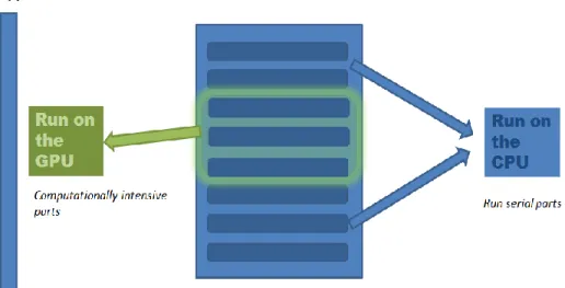
Figure 3: Program word division between the CPU and the GPU ... 3

Figure 4: High performance GPUs NVIDIA’s Tesla (left) and AMD’s FireStream (right) [77] .... 4

Figure 5: Intel’s Xeon Phi coprocessor [83] ... 5

Figure 6: GPU hardware architecture for the Fermi platform . There are 16 SMs (vertical rectangular blocks) [45] ... 8

Figure 7: Fermi SM architecture [45] ... 8

Figure 8: Kepler GPU hardware architecture [46] ... 11

Figure 9: Kepler SMX hardware architecture [46] ... 12

Figure 10: Maxwell SMM hardware architecture [79, 87] ... 14

Figure 11: Nvidia’s Kepler vs. Maxwell [87]... 15

Figure 12: CUDA kernel compilation process ... 16

Figure 13: CUDA memory model [36] ... 18

Figure 14: Particle exchange in the Grand Canonical Simulation ... 26

Figure 15: Gibbs ensemble moves ... 28

Figure 16: High and low angle grain boundaries ... 35

Figure 17: (a) A hexagonal lattice (b) A pentagonal and heptagonal lattice; each forms a disclination ... 37

Figure 18: GOMC flowchart ... 39

Figure 19: GOMC I/O compatibility with file formats used by other simulation engines ... 40

Figure 20: Radial cutoff (rcut) in a displacement move ... 42

Figure 21: Energy calculation mapping algorithm across threads ... 47

x

Figure 23: 2D View of a Conventional Cell List... 50 Figure 24: Using a microcell data structure reduces the total volume being processed ... 53 Figure 25: Speedup of cell list implementations over the 1 core CPU brute force implementation ... 59 Figure 26: Speedup of microcell list over conv. cell list for molecule intermolecular interactions ... 60 Figure 27: Speedup for cell list implementations for system intermolecular energy interactions over 1 core CPU brute force for octane systems (8 interaction sites, rcut = 2.5σ) ... 61

Figure 28: Speedup for microcell list for system intermolecular energy interactions over conventional cell list for octane systems. (rcut = 2.5σ) ... 61

Figure 29: Speedup for cell list codes for system intermolecular energy interactions over CPU brute force for octane systems (8 interaction sites, rcut = 4.0σ) ... 62

Figure 30: Speedup for microcell list for system intermolecular energy interactions over conventional cell list for octane systems (8 interaction sites, rcut = 4.0σ) ... 62

Figure 31: Execution time in milliseconds for the best configurations of the conventional and microcell lists when running on a Phi cluster ... 69 Figure 32: Execution Time in milliseconds for the best configurations of the conventional and microcell lists when running on a multicore CPU cluster ... 69 Figure 33: Execution time in milliseconds for the best configurations of the conventional and microcell lists when running on a GPU cluster ... 71 Figure 34: PFC system flowchart ... 74 Figure 35: (a) ψ array plot representation using HDF (b) Regions (white) generated by the connected component algorithm (c) Final atom representation ... 76 Figure 36: Delaunay triangulations for detected atoms. The figure also shows a hexagonal lattice and two disclinations ... 77 Figure 37: (θ) angle for a hexagonal lattice computed against a reference line ... 77

xi

Figure 38: Circular average mechanism ... 79

Figure 39: Correlation length ... 80

Figure 40: Dislocation and disclination count ... 80

Figure 41: Dislocation and disclination density ... 81

Figure 42: structure factor ... 81

Figure 43: Moments vs. Time ... 84

Figure 44: Log-scale plot of moments_0 vs. Time ... 84

Figure 45: Log-scale plot of moments_x vs. Time ... 85

Figure 46: Extended area of the grains ... 87

Figure 47: Original area of the grains ... 87

Figure 48: Atom orientation ... 88

Figure 49: Grain identification and region buffers ... 88

Figure 50: Example on grain detection for a system of size 5122 at time 10000 (a) ψ plot (b) detected grains (c) grain boundaries detection ... 89

Figure 51: Grain identification for a system size of 5122 at time 15000 ... 90

Figure 52: Grain identification for a system size of 5122 at time 20000 ... 90

Figure 53 : Triple junction count ... 91

Figure 54: Average and maximum curvature of grain boundaries ... 92

Figure 55: Average and maximum velocity for grain boundaries ... 93

Figure 56: Average and maximum velocity for triple junctions... 93

Figure 57: Average and maximum angle misorientation of neighboring grain angles ... 94

Figure 58: Log-scale run time comparison for the g6 function ... 96

Figure 59: Log-scale runtime comparison for the PFC iterator simulation ... 97

CHAPTER 1 INTRODUCTION

This chapter will introduce coprocessors and their role in scientific research, focusing on GPUs as they are the main coprocessors used in this work. In addition, this chapter will give an introduction to the contributions presented in this work.

1.1 PC Coprocessors

For the last 40 years, microchip manufacturers have been developing computer processors that are designed to offload intensive calculations from the main processor to accelerate the system’s performance. Those processors are called coprocessors or sometimes accelerators. Coprocessors can be used to help process large floating point arithmetic, encryption, signal processing, and graphics. Many of the early coprocessors were designed to accelerate floating point tasks, such as the Intel 8087 coprocessor, and the Motorola 68881/68882 coprocessors [83].

The high competition in the gaming and movie industries resulted in the introduction of high performance graphics cards that provide superior processing capabilities while being affordable at the same time. Graphics processors were considered as coprocessors for generating visual output; however, with all these processing capabilities, researchers have been interested in using them in applications that were infeasible in the past because of their long execution times and the unavail-ability of inexpensive supercomputers.

To render movies and game scenes, pixels are drawn in parallel by creating a multithreaded program that uses each thread to render different pixels [1]. This parallel architecture was the foundation for using the graphics processors for more general applications or what is commonly called GPGPU (General-Purpose Graphics Processing Unit) programming [1]. Along with the introduction of GPGPU programming came the development of specialized programming lan-guages and APIs that provide a clear and flexible framework to write programs that run on graphics processors such as CUDA (Compute Unified Device Architecture), which was created by NVIDIA [2].

Figure 1: Floating point comparison between the GPU and CPU [6]

GPUs offer unprecedented performance and they are designed to have high throughput. The GPU performance is rapidly increasing compared to CPU performance. Figure 1 shows a histori-cal comparison between different types of CPUs and NVIDIA GPUs in terms of floating point operations per second (FLOPS/s) [6]. In addition, the memory bandwidth of GPUs is also increas-ing rapidly compared to CPUs as depicted in Figure 2 [6].

GPUs are now becoming a preferred choice to accelerate simulations in many fields of science as they are available and cheap relative to other types of high-performance computing options. GPUs have hundreds or thousands of processing cores compared to only a few in most CPUs, and this is why GPUs have high computational throughput [2]. Many GPU programming research projects have been conducted in different science fields [78]. GPUs are developing very quickly, as it can be noticed from Figures 1 and 2, and in the near future more features will be added to them to help in producing more energy efficient programs and to ease the conversion from se-quential codes to parallel codes [107].

Figure 4: High performance GPUs NVIDIA’s Tesla (left) and AMD’s FireStream (right) [77]

GPUs offer high performance if there is sufficient parallelism for them to be used to process the most computationally intensive portions of the application. CPU code is generally going to handle other portions of the application, such as I/O and program flow control because GPUs do not have direct access to I/O devices, and the CPU has more complicated cache management and control prediction than GPUs. Figure 3 shows how an application can be divided between the CPU and GPU.

While there are many hardware manufacturers for GPUs, the main two GPU manufacturers are NVIDIA and AMD. GPUs manufactured by those two companies are used now in all kinds of computers, from smartphones all the way up to supercomputers. Examples of supercomputers that are using GPUs are Titan at Oak Ridge National Laboratory, which has 18,688 NVIDIA K20X GPUs providing a theoretical peak performance of 27 petaflops [3]. Both companies produce high end GPUs for scientific applications. Figure 4 shows an Nvidia Tesla and an AMD FireStream GPUs, where both GPUs are designed to run high demanding scientific applications.

Early GPUs used programming languages such as OpenGL and Microsoft’s DirectX [1]. However, many GPU programming languages were hard to learn and use, and lacked the repre-sentation of many operations that are needed, such as arithmetic operations. Modern GPUs are being programmed mainly by two programming frameworks, the open cross-platform OpenCL [4], and Compute Unified Device Architecture (CUDA) from NVIDIA [5].

In 2012, Intel introduced the Xeon Phi coprocessor. This coprocessor is an SMP (Symmetric multiprocessing) on a chip [83] that runs Linux OS. The Knights Corner Phi coprocessor has 61 cores, and 4 hardware threads per core. Phi coprocessors can run single and double precision cal-culations. The Cores have also L1 and L2 caches, vector processing unit, and scaler unit [83]. The super computer Tianhe-2 has 48,000 Xeon Phi 31S1P coprocessors [84]. Figure 5 shows an active Xeon Phi processor (left) and a passive one that is cooled externally (right).

Figure 5: Intel’s Xeon Phi coprocessor [83]

1.2 Programming Coprocessors

There are many frameworks that are used to program accelerators, such as OpenCL [4], OpenACC [86], CUDA [6], and OpenMP [85]. Message Passing Interface (MPI) is language in-dependent standard that is used to pass data between connected coprocessors or CPUs. There are

many implementations of MPI standards, and some are free and open source [105]. MPI has many functions to do data collection and synchronization [105]. MPI can be used with other ac-celerator programming standards to program heterogeneous acac-celerator clusters [85, 105].

OpenCL can be used to program parallel applications that can run across heterogeneous sys-tems. Many hardware manufacturers adopted this open standard, such as Nvidia, AMD, Apple, IBM, and Samsung [4]. OpenCL provides a low-level programming framework that can achieve good performance, but using OpenCL can produce less portable code when it is used to write ap-plications for a specific hardware.

OpenMP (Open Multi-Processing) is another framework that provides a set of APIs to be used to parallelize programs [85]. A main thread usually forks into a number of sub threads that can be used to process the work load simultaneously. There are APIs to identify threads, sum data from threads, and synchronize threads.

OpenACC (Open Accelerator) [86] is a new programming standard that aims to provide more support for programming heterogeneous platforms. OpenACC has high-level directives that can be used to parallelize loops and optimize data locality.

CUDA (Compute Unified Device Architecture) [6] is a proprietary parallel programming framework that is developed by Nvidia. CUDA can only be used to program Nvidia’s GPUs. Nvidia designed CUDA to work with C, C++, and FORTRAN, which makes it easier to use. As it can only run on Nvidia’s GPUs, CUDA has many functions that could be used to exploit the hardware features of those GPUs.

1.3 GPU Technology Development

Before GPUs, many computer hardware manufacturers introduced graphics controllers that were used to accelerate graphics drawing. Some of the graphics controllers had general purpose languages that can be used to write general purpose programs; however, they were very hard to learn and use.

Throughout the 1980s and 1990s, graphics controllers continued to evolve, and 3D graphics cards were introduced to meet the increasing demand for more realistic and high resolution games and movies [3, 6]. In 1999, NVIDIA introduced the GeForce 256 graphics card, which is consid-ered to be the first consumer-level graphics processing unit (GPU) [1, 2] that had integrated the capabilities of rendering 3D images in real time, and a programmable framework for parallel pro-gramming in a single chip.

With the introduction of the GeForce 256, the term GPU became popular and other manufac-turers adopted the name or introduced similar terms. After that, GPU technologies continue to evolve, and new GPUs are consistently introduced that have better capabilities than before in terms of number of processing cores, memory, bus speed, and core clock rate.

1.3.1 GPU Architecture

The latest architecture introduced by NVIDIA is the Maxwell [79, 87] architecture, which was released in February 2014. However, many of the current GPUs are still built on the previous Kepler [46] and Fermi [45] architectures.

1.3.1.1 Fermi Architecture

The Fermi architecture was introduced in 2010 [45], and came with many major improve-ments over the earlier Tesla architecture. Figure 6 shows the main hardware components for the Fermi GPUs, while Figure 7 shows the Streaming Multiprocessor (SM) architecture.

The basic building blocks for a Fermi GPU are: 1- Streaming Multiprocessors (SMs):

The SMs are the main processing blocks on the Fermi GPU. Each SM has 32 CUDA cores in hardware revision 2.0, and 48 cores in the hardware revision 2.1. A CUDA core is a proces-sor that is equipped with a pipelined arithmetic logic unit (ALU) and a floating-point unit (FPU).

Figure 6: GPU hardware architecture for the Fermi platform . There are 16 SMs (vertical rectangular blocks) [45]

Each SM can perform up to 16 double-precision operations per clock cycle, which is a considerable improvement over the previous architecture. This improvement helps in doing more accurate simulations.

Load/Store (LD/ST) units are responsible for calculating the source and destination ad-dresses for the memory. Having sixteen of those (LD/ST) units on board a Fermi GPU will enable threads to do sixteen (load/store) address calculations per clock cycle [45]. In addition, each SM has four special function units (SFU) that can be used to execute some math func-tions such as sine, cosine, and square root [45].

To handle thousands of threads, the GPU follows the single instruction multiple data (SIMD) model. Threads are scheduled in batches of 32s called warps [3]. To organize the exe-cution of thread warps, the Fermi GPU has a dual warp scheduler. At each clock cycle, each scheduler will select an instruction from a warp and assign it to a group of 16 processors or the four SFUs. Integer, float, load/store, and SFU instructions can be dual issued, while double precision instructions cannot be dual issued.

Another improvement over the previous architecture is having a full hierarchy memory, with shared memory and an L1 cache that share 64K on each SM.

2- Memory Hierarchy:

There are different types of memory that can be used in CUDA. Memory types differ in bandwidth, access rate, and size. The main types of memory in CUDA are:

a. Global memory: The global memory is the largest memory on the GPU; however, it is the slowest memory. The global memory can be used to share data between all threads on the device. To achieve efficient memory accesses, data reads and writes should be coalesced.

b. Shared memory: The shared memory is an on-chip memory that is faster than the global memory. Shared memory can be used to share data between threads in the same thread block. However, bank conflicts can decrease the access speed to data in

shared memory. Bank conflicts can be reduced by distributing the values in shared memory so that each thread in a warp either accesses the same shared memory value or values in different banks. Since memory is allocated among the banks in 4-byte in-crements, a double spans two adjacent shared memory banks.

c. Registers: Registers are the fastest memory type on the GPU; however, they are lim-ited in number and size. Registers are used to store local variables in a kernel, but if there are not enough registers to store all the local variables, global memory will be used to store those variables.

d. Constant memory: Constant memory is a 64 KB read-only memory that is used to store constants. Only 8 KB is cached on an SM.

e. Texture memory: Texture memory is a cached read-only memory that is optimized for 2D spatial locality. Threads that belong to the same warp that access nearby tex-ture memory locations will get better memory access performance.

3- Error Correcting Code (ECC):

Data inside memory can be altered by outer factors such as radiation, so the Fermi archi-tecture added an ECC unit that detects and corrects such errors.

4- GigaThread Thread Scheduler:

At the chip level, Fermi schedules threads at a global level by distributing thread blocks to different SMs. Fermi GPUs also introduced many more improvements such as faster atomic operations, enhanced reductions, faster context switching, support for concurrent kernel exe-cution, and improved branch prediction.

1.3.1.2 Kepler Architecture

Kepler came with many improvements over the Fermi architecture in terms of throughput, memory bandwidth, and power consumption [46]. Figure 8 shows the Kepler GPU architecture. New features of the Kepler GPUs include:

1- The new Streaming Multiprocessor (SMX) Architecture:

SMs in the Kepler architecture have far more cores and capabilities than the Fermi ar-chitecture. Figure 9 shows the Kepler SMX arar-chitecture. The first thing to be noticed is the number of CUDA cores per SMX has been increased to 192. A major improvement in the double-precision support is an increase in double-precision units. Now, there are 64 double-precision units in each SM. In addition, there is an 8-fold increase in SFU units, and a 4-fold increase in LD/ST units [46].

Figure 9: Kepler SMX hardware architecture [46]

Another major improvement is the introduction of two more warp schedulers, which means that four warps can be issued and executed concurrently. Moreover, each Kepler warp scheduler is now equipped with two instruction dispatching units, allowing for more concurrent execution. In addition, double-precision instructions can now be dual issued.

Other improvements include the introduction of the shuffle instruction that allows threads belonging to the same warp to share registers, an increase in the number of regis-ters per thread, the ability to configure shared memory for 8-byte banks for increased bandwidth and better support for double-precision numbers, the expansion and accelera-tion of atomic operaaccelera-tions, and an increase of the GPU texture memory throughput. 2- Dynamic Parallelism:

In Fermi, the GPU cannot generate new work unless the CPU does that for it. In other words, all kernels are launched by the CPU. In Kepler, a new concept called dynamic parallelism was introduced to enable the GPU to launch kernels by itself, independent of the CPU. By using dynamic parallelism, the GPU can adapt the flow of the kernel execu-tions and launch the required number of threads directly.

3- Memory Enhancements:

Kepler has a similar memory hierarchy to Fermi; however, Kepler enables the use of the read-only 48 KB data cache that was only accessible by the Texture Unit in Fermi. In addition, shared memory and L2 cache bandwidths are doubled.

Additional Kepler improvements include support for multiple CPU cores to launch work on the same GPU by introducing Hyper-Q, and direct GPU access through the network without go-ing through the CPU memory by introducgo-ing GPUDirect [46].

1.3.1.3 Maxwell Architecture

The latest architecture from NVIDIA is the Maxwell architecture [79]. The main goals of troducing this new architecture are to develop GPUs for smaller computer platforms, and to in-crease performance while consuming less power. Figure 11 shows that the performance per Watt doubled compared to the previous Kepler architecture, and the performance per core is 35% more than in Kepler. To achieve those goals, NVIDIA introduced a new streaming multiprocessor ar-chitecture called SMM [79]. The new SMM is designed with more L2 cache and shared memory to improve performance; in addition to a group of architecture design changes that enable the Maxwell architecture to achieve double the performance for the same amount of power compared the Kepler architecture [79]. For instance, the new SMM uses four control logic units to dispatch the instructions, as shown in Figure 10, and the number of active threads per block increased from 16 in Kepler to 32 in Maxwell. In addition, new improved algorithms are designed to enhance the scheduling process. However, there are no high-end GPUs manufactured on the Maxwell archi-tecture yet. More information on the Maxwell archiarchi-tecture can be found in [79, 87].

Figure 11: Nvidia’s Kepler vs. Maxwell [87]

1.3.2 GPU Programming

While OpenCL is used to program different GPU architectures, CUDA runs only on NVID-IA’s GPUs. CUDA also provides a large number of libraries [6] that are optimized for its GPUs such as:

- cuFFT: Library for Fast Fourier Transformations. - cuBLAS: GPU accelerated BLAS library.

- cuSPARSE: GPU functions for sparse matrix operations. - Thrust: Open source library of different data structures. - cuRAND: GPU accelerated random number generator.

In addition, CUDA provides more built-in features and functions, supports templates, and has more support for developers. A showcase of CUDA libraries can be viewed at [7]. The main drawback of CUDA is that it is not an open standard. Since OpenCL is an open standard, it can be used on AMD GPUs, NVIDIA GPUs, and Intel Xeon Phi co-processors, along with other multi-core platforms.

CUDA simplifies many operations that were very hard to implement using earlier GPU pro-gramming languages, and provided a list of instructions to support parallel propro-gramming, thread management, synchronization, and memory management [6]. Figure 12 shows how CUDA com-piles the CPU and GPU integrated codes.

1.3.2.1 Synchronization in CUDA

Synchronization is an important feature in any parallel programming framework. As threads execute in parallel, there is no guarantee on the order in which they will be executed. Hence, syn-chronization is needed to organize the execution of parallel programs. CUDA provides a set of synchronization tools for programmers.

Figure 12: CUDA kernel compilation process

CUDA kernels are launched asynchronously; thus, after the host launches a kernel, the CPU will continue with the program execution. In some cases, results from the kernel are necessary for making decisions or generating output. As a result, CUDA has a statement called

cudaDevic-eSynchronize() [6]. cudaDeviceSynchronize will block the host until the kernel is finished exe-cuting. However, memory copy statements after the kernel launch will also block the host without requiring an explicit synchronization statement.

To synchronize threads in a thread block, CUDA has the __syncthreads() [6] statement. CUDA did not implement a function for cross-block synchronization because it can be costly in terms of performance. There are ways to do it programmatically by using atomic operations as locks, but again it can degrade performance.

CUDA also provides memory fence functions such as __threadfence() [6] and _threadfence_block() [6]. When a thread calls the __threadfence() function, it will block until all its previous writes to global memory and shared memory are visible to all other threads. The __threadfence_block() [6] instruction works the same way as __threadfence(), but on a block lev-el.

1.3.2.2 Kernels and Device Functions

The main units of code execution on the GPU are called kernels. Kernels are created by put-ting the __global__ directive before the function definition. An example of a kernel function def-inition is:

__global__ void MyKernel(parameters)

Kernels cannot have a return type because they cannot return values directly. The only way of returning values is to use memory copy functions. To launch a kernel, the programmer should specify the number of threads per block and the number of blocks, and provide the function ar-guments. In some cases, kernels may have dynamic shared memory, so the programmer must also provide the size for that memory space. A kernel call would look like this:

MyKernel<<<Grid Size, Block Size>>> (arguments)

CUDA threads are organized into thread blocks, and blocks are organized into a grid. Threads inside a thread block can be organized into one, two, or three dimensions, with a limit of 1024 threads per block on most GPUs. Blocks within a grid can be organized into one, two, or three

dimensions. This flexibility in thread and block organization can be very useful in applications that have multidimensional data. Figure 13 gives a view of how threads, thread blocks, and grids relate to each other. By having threads divided into thread blocks, the hardware can scale the exe-cution of the kernels to any GPU without the need to change the code.

When a kernel is launched, the grids are assigned to SMs to be executed. A thread block is as-signed to one SM, and an SM can have more than one block asas-signed to it depending on how many threads are in that thread block. Registers and shared memory are also partitioned among threads and thread blocks.

1.3.2.3 CUDA Memory Model

Threads inside a thread block can communicate using shared memory. Shared memory pro-vides a fast way for threads to share data. Each thread can store local variables inside registers. However, shared memory and registers are limited in size, so to store large data structures; the GPU uses the global DRAM memory, which is the slowest type of memory on the device. Care-ful planning of the use of the memory types and how data is partitioned among them can enhance performance. Figure 13 shows the CUDA memory model and how it is related to threads and thread blocks.

1.3.2.4 GPU-CPU Communication

Data is transferred into and out of the GPU by using memory calls [2]. Those memory calls can affect performance if not used carefully. Data can also be moved asynchronously between the GPU and CPU by using asynchronous memory calls. Data transfer between the CPU and the GPU is very time consuming, and thus should be reduced to a minimum.

1.3.2.5 Functions and Libraries

CUDA provides many libraries that are GPU optimized. In addition, CUDA provides a set of alternative math functions called intrinsic functions [28]. Intrinsic functions are faster than stand-ard math functions in CUDA; however, they are less accurate. These functions may be used in calculations that can tolerate some loss in accuracy to gain more speedup. In addition, there is a set of atomic instructions that can be used to provide locks on data when it is modified. Examples of atomic functions are atomicAdd, atomicSub, atomicDec, and atomicAnd [28].

1.3.2.6 Compute Capability

In CUDA, the compute capability specifies the architecture of the GPU, described in terms of major and minor revision numbers. When two GPUs have the same major revision number, then this indicates that they have same architecture. The current major revision numbers are one, two, three, and five corresponding to Tesla, Fermi, Kepler, and Maxwell architectures, respectively.

The minor revision number specifies improvements that are made on the same architecture. More details on what capabilities each one of the CUDA compute capabilities have can be found in [6].

1.3.2.7 CUDA Streams

One of the powerful concurrency features of CUDA is CUDA streams. A stream is a sequence of instructions that are executed in the order that they are issued on the GPU [2, 28]. By default, there is one stream that the kernels are launched through. CUDA streams are used to achieve con-currency beyond the multithreading level. Instead of executing one kernel at a time on the device, CUDA streams can be used to execute a number of kernels concurrently on the device, which can be used to introduce more speedup. However, the ability to run multiple kernels concurrently de-pends on the device, which in this case should be of compute capability 2.0 and up. Another fac-tor that is important is the availability of resources on the device. If each kernel uses a lot of hardware resources, then there will not be enough resources to run multiple kernels concurrently.

1.4 Research Contributions

The two research projects presented in this dissertation are: the development of an open-source Monte Carlo GPU code for thermodynamic ensemble interactions called GPU Optimized Monte Carlo (GOMC) [70], and the development of a GPU code for accelerating the computation of polygrain growth in the Phase-Field Crystal (PFC) [112, 113] model.

GOMC is an NSF-funded interdepartmental project with Professor Jeffrey Potoff’s research group from the Department of Chemical Engineering and Materials Science. The GPU PFC pro-ject is also a joint propro-ject with Professor Zhi-Feng Huang from the Department of Physics and Astronomy. The enhancement of their software to run on the GPU is an important step for in-creasing the problem size and features of the systems, both of which allow deeper scientific un-derstanding of the behavior of these systems.

Monte Carlo (MC) simulation has been used to study many problems in statistical physics and statistical mechanics that are not possible to simulate using Molecular Dynamics (MD) [8]. One

example is the simulation of adsorption of gases in porous materials [8]. While there are a fair number of well-known and widely used GPU Molecular Dynamics codes, such as LAMMPS [9], NAMD [10], AMBER [11], and HOOMD Blue [12], the existing Monte Carlo ensemble simula-tions are relatively slow and so are not practical for simulating large systems. In addition, those Monte Carlo codes are not yet ported to the GPU, which makes it almost impossible for research-ers to run large systems in a reasonable amount of time. GOMC is created to address these short-comings of existing Monte Carlo ensemble codes.

There are many challenges I faced when developing the GOMC GPU Monte Carlo molecular simulation. For instance, data structures need to be designed to enable memory coalescing for GPUs, the use of different techniques to optimize the ways to calculate energy interactions for the GPU, when and what data needs to be copied from and to the GPU, how to enable the code to scale when executed on more than one device, and the ability of the code to simulate systems with different types of molecules. Through this work, I introduced many optimizations that tar-geted those challenges.

The GPU PFC modeling is motivated by recent research efforts devoted to the understanding of the properties of crystalline materials, both their design and control. Recent developments in-clude the introduction of new models to simulate system behavior, and novel properties that are of significant experimental and theoretical interest. One of those models is the Phase-Field Crys-tal (PFC) model [112, 113]. The PFC model has enabled researchers to simulate 2D and 3D crys-tal structures and study defects such as dislocations and grain boundaries. In this work, the Multi-core Computing Lab carries out large-scale computer studies on GPUs to examine various dy-namic properties of polycrystals in the 2D PFC model. Some properties, such as the Orientational Correlation function (g6) [26, 35], require taking the circular average over different radii for every

atom. This is very compute intensive when the system has hundreds of thousands of atoms. This thesis reviews related work on both the GOMC and PFC projects in Chapter 2. Chapter 3 will describe the GOMC main components, flowchart, data structures, how energy interactions

are implemented and optimized using the cell list structure, and finally present and discuss the results. Chapter 4 will go over the PFC model, how the model was implemented and optimized for running on GPUs, the calculation of different PFC related properties, and finally present and analyze the performance of the PFC solver and different properties that run on the GPU. Finally, Chapter 5 will present the overall conclusions from this work, and what are the future contribu-tions that I am planning for the two research projects.

CHAPTER 2 RELATED WORK

This chapter will present an overview of the Monte Carlo simulations, giving details on the ensembles programmed in this work, and how they are calculated. In addition, the chapter will go over grain growth, while focusing on the PFC model that is used in this work. The chapter will also present related work on some well-known Monte Carlo molecular simulation engines.

2.1 Monte Carlo (MC) Simulations

MC methods are a set of stochastic methods that use random numbers and probability statis-tics for problem investigation [16]. Through the use of repetitive random sampling on the input domain, then processing the selected inputs, MC methods try to converge to a steady-state solu-tion. There are many applications of MC methods in the fields of physics, finance, artificial intel-ligence, and biology [8, 17, 19].

One of the applications of the MC method is the simulation of molecular systems. A popular MC model that is used to simulate such systems is called the Metropolis method [17]. The Me-tropolis method is used to evolve the system through multiple iterations that consist of selecting particles or molecules, performing a type of interaction with that selected particle or molecule, calculating the energy change, and then deciding based on a random value whether or not to ac-cept that interaction. The Metropolis main steps are:

1- Generate initial system configuration.

2- Perform a move, such as particle displacement. The particle should be chosen and dis-placed randomly.

3- Calculate the energy change (ΔE) for the displaced coordinates. 4- Decide whether to accept the move or not:

b. Else, calculate 𝑒(−

𝛥𝐸

𝑘𝑇)_{, and draw a random number R from the [0,1) range. If R >}

𝑒(−𝛥𝐸𝑘𝑇) _{then accept the new coordinates. Else, reject the move and keep the old}

coordinates. In either case, return to step 2.

2.1.1 Statistical Thermodynamics Ensembles

One of the MC applications of molecular systems is the thermodynamic ensemble simulation [8, 19]. Ensembles represent the thermodynamic properties of a system. This work focused on the following three main ensembles, canonical ensemble, grand canonical ensemble, and Gibbs en-semble.

2.1.1.1 Canonical Ensemble

Canonical ensemble is one common ensemble in which the number of molecules or particles (N), box volume (V), and temperature (T) are fixed, so sometimes it is referred to as NVT [18]. NVT can simulate two moves, molecule or particle displacement, and molecule rotation.

Acceptance criteria are measured by using the Boltzmann factor given by:

𝑒−𝛽∆𝐸 _(2.1)

where ΔE is the energy change between two states, and βis equal to 1 (𝑘⁄ _𝐵𝑇), where kB is the Boltzmann constant and T is the temperature in kelvin [18].

To calculate the Boltzmann factor for a move, ΔE needs to be calculated, which represents the change in energy between the old and new positions. After the Boltzmann factor is calculated, the result will be compared against a random number drawn uniformly from the [0,1) range. If the Boltzmann factor result is larger than the drawn random number, the move will be accepted, and the new coordinates are committed. NVT pseudo-code is shown in algorithm 1.

Algorithm 1: Canonical ensemble pseudo-code

Canonical Ensemble Algorithm

input: steps, Number of particles , Volume, Temperature // Calculate the system’s initial energy

// Main Loop for i := 1 to steps do

// Randomly select a particle to move s ← rand()

Old_particle_loc := particle_location(s) // Randomly move to a new location New_particle_loc := randCoords()

// Calculate the selected particle’s energy for the old and new locations for k := 1 to number of particles do

if k!=s then old_energy_contrib ‏+= calculate_pairwise_energy(Old_particle_loc, k) new_energy_contrib ‏ += calculate_pairwise_energy(New_particle_loc, k) end if end for deltaE := new_energy_contrib–old_energy_contrib. calculate_acceptance_rule() if accepted then total_energy ‏ += deltaE current_config := new_config update_system_status() end if updateMoveStatistics()

//Solve if the system in equilibrium state // Periodically write system status to disk end for

2.1.1.2 Grand Canonical Ensemble

The grand canonical ensemble extends the canonical ensemble by defining temperature, vol-ume, and the chemical potential as constants [18]. A reservoir is connected to the simulated sys-tem, allowing the particles and energy to be exchanged freely between them. Through this ex-change of particles, the system and the reservoir will reach an equilibrium state, which can be determined by using the fixed values of the temperature and the chemical potential.

Figure 14 gives an example of a grand canonical simulation that has the simulated system with V volume (N particles), and the reservoir with V0-V volume (M-V particles). Particles can

inter-act with each other only when they exist inside the simulated system. The grand canonical pseu-do-code is shown in algorithm 2.

Algorithm 2: Grand canonical ensemble pseudo-code

2.1.1.3 Gibbs Ensemble

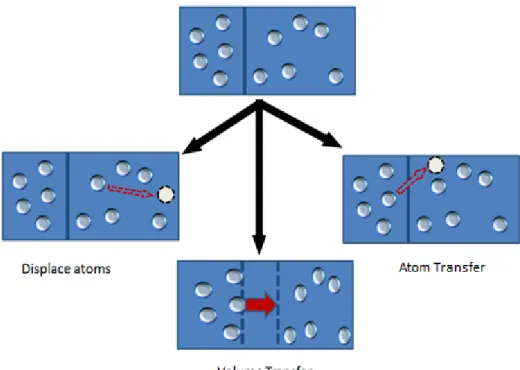
Gibbs ensemble is used to simulate phase equilibria in vapor-liquid coexistence systems. In addition, Gibbs ensemble can be used to simulate many more systems such as solid-fluid equilib-ria, solid-vapor equilibequilib-ria, adsorption equilibequilib-ria, and membrane equilibria [36].

To model coexistence systems, we need to have two boxes. A series of moves can then be per-formed on those boxes, which include:

1. Particle or molecule displacement within a box:

Grand Canonical Ensemble Algorithm

Input: steps, Number of particles, Volume, Temperature, Infinite Reservoir //Initialize particles’ coordinates inside the box randomly

// Calculate the system’s initial energy //Main simulation loop

for i= 1 to steps do

//Randomly select a move type R ← rand()

if (R < DisplacePercent) then

//Attempt particle displacement

else

//Attempt particle transfer (Insertion/Deletion)

//Choose a random source (Box or Reservoir)

Source ← rand()

if (Source < 0.5 ) then

//Source box is the Box remove a random particle)

else

//Source box is the reservoir (Insertion a new particle to the box)

end if

end if

//Solve if the system in equilibrium state //Periodically update system status to disk end for

This move is the same move used in canonical and grand canonical ensembles. 2. Volume transfer:

Transfer an amount of volume from one box to the other. 3. Molecule or particle transfer:

An particle or molecule can be transferred from one box to another. However, there are different ways to do this.

Figure 15 shows an illustration of the Gibbs ensemble moves. Algorithm 3 gives the Gibbs en-semble pseudo-code.

Figure 15: Gibbs ensemble moves

2.1.1.4 Configurational Bias

Sampling chain-molecules in MC simulations is a very important issue to achieve configura-tional equilibrium. A great deal of research has been devoted to the development of efficient methods to sample different structures for chain molecules; however, many of those methods will not work in dense systems [19]. One way to address the sampling problem is to completely

re-build the whole molecule or parts of it, while biasing the re-build toward preferable configurations. This method was proposed by Siepmann and Frenkel [19], and it was named configurational bias MC (CBMC). CBMC is based on the self-avoiding random walk algorithm that was proposed by Rosenbluth.

CBMC starts by choosing different random positions for the next particle to build. Those posi-tions must not be occupied by any other existing particle in the system. For each generated trial position, one needs to calculate the Rosenbluth weight [19].

Algorithm 3: Gibbs ensemble pseudo-code

Gibbs Ensemble Algorithm

Input: steps, Temperature, Two boxes of volume (V1,V2) and number of particles (N1,N2)

//Main simulation loop for i = 1 to steps do

// Select a move type randomly

R← rand()

if (R < disp_percentage) then

//Attempt particle displacement move //Select a box randomly

selectedBox← rand()

// Attempt to displace an particle in the selected box

else if ( R < (disp_percentage + vol_percentage ) ) then

// Attempt Volume Transfer

else

//Attempt particle transfer

//Randomly select a source box sourceBox ← rand()

// perform an particle transfer move to the other box end if

//Solve if the system is in equilibrium state //Periodically write system status to disk

end for

To achieve detailed balance [19], the trials are done at both boxes, where the trials at the source box are referred as old trials. As we build new sites, old and new trial weights are accumu-lated and used in the end to accept or reject the move. More on CBMC can be found in [19, 27].

2.1.2 Lennard-Jones Potential

The Lennard-Jones potential is a mathematical approximation used to compute the energy in-teraction between a pair of particles or molecules that incorporates the attractive and repulsive forces [8, 36]. The Lennard-Jones potential calculation is done using the following equation:

𝑉_𝐿𝑗 = 4𝜖 [(𝜎_𝑟)12− (𝜎 𝑟)

6

] (2.2)

where σ is the particle diameter, ϵ is the well depth, and r is the distance between the two par-ticles.

2.1.3 Calculating Force Interactions

Other simulation techniques, such as molecular dynamics, typically require significantly more computation for each step of the simulation, and so are better-suited for parallel implementation. Even so, some previous simulations have used the GPU to implement the MC method [51]. Their implementation depends on an embarrassingly parallel algorithm that runs several concurrent simulations with small systems of 128 particles. Instead, this work uses the energy decomposition method (farm algorithm), which enables us to support configurations with over a million parti-cles. In [61], a parallelization method for the canonical MC simulations via domain decomposi-tion technique has been presented, where each domain can be assigned to a separate processor and multiple moves can be simulated in parallel. Interprocess communication is required only when moving particles near the edge of a domain, since this requires interactions between adja-cent domains. To limit this communication, each domain is partitioned into three subdomains. The size of the middle subdomain is chosen as large as possible to minimize interprocess com-munication. Although well suited for a multicore CPU, this approach does not expose the

fine-grained parallelism required for an efficient GPU implementation. Each time a particle is dis-placed in, removed from, or inserted into the simulation region, energetic decomposition requires that pairwise energy be calculated between this particle and all other particles. A radial cutoff, denoted as rcut, is typically chosen to reduce the execution time by limiting the calculation of

in-ter-molecular forces to only those particles within the cutoff. The forces due to interactions with particles outside of the cutoff can be approximated using tail corrections [18]. Since interactions within only a small radius are considered, it is possible to create either a cell list or a neighbor list to organize particles based on their relative locations and ignore particles that are beyond the cut-off. In this way, not only are the energy and pressure computations of more distant pairwise inter-actions avoided, but also the calculation of distances between these particles.

Another approach to calculating force interactions between particles is based on reducing or eliminating the interactions with particles that are beyond the cutoff by constructing a neighbor list or a cell list. One common example of the neighbor list is the Verlet list [89]. Verlet lists maintain a list of neighboring particles for each particle, where those neighboring particles all fall within the cutoff. While this list reduces the number of interactions that must be computed, it re-quires more frequent updating. For MD, the Verlet list is a good option, as all particles move simultaneously and the system is closed in terms of adding or deleting particles [90]. In contrast to MD, the MC system is open, and particles can be displaced for relatively large distances, which may sometimes require rebuilding the whole Verlet list.

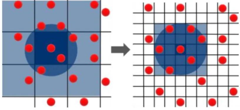
In the conventional cell list approach [91], the simulation box is divided into cells (squares in 2D, cubes in 3D) such that the dimensions of each cell are greater than or equal to the cutoff. Here, the cells will limit the number of interacting particles by only considering interactions across adjacent cells. However, adjacent cells may still have particles that are outside the cutoff, thus there is a need to check all pairwise interactions in adjacent cells. When compared to Verlet lists, cell lists require less effort to maintain, especially when displacing or deleting particles. To reduce the number of extraneous processed interactions in the cell list approach, cell dimensions

may be selected to be smaller than the cutoff, or in some cases, make the cell small enough to fit only a few particles [92]. However, this approach will generate many fine-grained cells that need to be examined, and in sparse boxes, many of those cells will be empty [92]. MC simulations per-form much less computation at each step when compared to MD, so approaches that show good performance for MD simulations using cell lists and Verlet lists did not yield performance gains when simulating small systems for MC interactions [92].

There are many examples of using a cell list implementation for the MD simulations [18, 47, 65, 93, 94]. On early GPUs, an efficient implementation of cell list on the GPU was not viable due to the lack of atomic operations on the GPU [51]. Instead, implementations such as [65, 93, 94] use the CPU to construct the cell list and then copy it to the GPU. These cell lists are then used to construct a neighbor list. Note that in molecular dynamics simulations, all molecules are moved in each step, requiring the cell list to be updated after nearly every simulation step. The frequency of updates depends on how far a molecule moves in each step, how much extra dis-tance beyond the cutoff is used in defining the neighbors, and how much inaccuracy can be toler-ated in the computations. A state-of-the-art implementation is described in [12].

A third option is to use both a Verlet list and a cell list [95]. For instance, Proctor et al. [90] show cell lists on the GPU allow a fast approximation of whether or not two particles are within the cutoff, which performs better than immediately traversing the neighbor list. They do not cre-ate or maintain a cell list, but calculcre-ate the cell of each particle based on its coordincre-ates, with cell dimensions larger than the cutoff, and use this calculation to determine whether or not two parti-cles are in neighboring cells.

2.1.4 Molecular Simulation Engines

Molecular Dynamics (MD) and Monte Carlo (MC) computer simulations are the most widely used simulations in materials science.MD codes have been considered as better candidates for parallel implementation because each simulation step in a MD simulation requires considerably huge computation effort when compared to MC simulations. For this reason, many molecular

dy-namics codes have been developed, some of which have been modified to utilize the GPU, in-cluding LAMMPS [9], NAMD [10], AMBER [11], and HOOMD-Blue [12]. On the other hand, there is a class of problems that cannot be simulated using the current methodologies. For exam-ple, adsorption in porous materials is the sort of problem that requires the simulation of an open system, which requires a methodology that allows for fluctuation in the number of molecules in the system.

While MD simulations have been studied well by other researchers, other systems are impos-sible to simulate using these MD codes, such as the simulation of multicomponent adsorption in porous solids [97], which will open the door for solutions such as the development of novel po-rous materials for the sequestration of CO2 and the filtration of toxic industrial chemicals. In

par-ticular, molecular dynamics (MD) codes cannot be used to simulate an open system without using a hybrid MC-MD approach [89, 99] because of the fluctuation property of MC that MD does not utilize.

Another general purpose molecular simulation is the HOOMD-Blue (Highly Optimized Ob-ject-Oriented Many-Particle Dynamics) simulation engine that is developed in Michigan State University. HOOMD-Blue is programmed to use GPUs to accelerate MD simulations, and it can scale up to thousands of GPUs, thus enabling it to perform very large simulations [12]. There is MC extension for HOOMD-Blue that is called Simpatico [100] that supports some MC algo-rithms. Another extension for HOOMD-Blue is called Hard Particle MC (HPMC) [41], which supports doing MC hard particle simulations [41].

Sandia National Labs started developing an open source simulation engine for MD simulation in 1995, which has the capability to run on parallel processors. The simulation engine is called LAMMPS (Large-scale Atomic/Molecular Massively Parallel Simulator) [9]. LAMMPS can be run on many modern parallel accelerators, such as GPUs and Phi coprocessors. To improve effi-ciency and enhance performance, LAMMPS uses neighbor lists to track of close particles [9].

Loyens et al. [57] developed a parallel MC Gibbs ensemble simulation that specifies algo-rithms to parallelize each movement type of the MC simulation. For displacement, the system can be divided into regions, provided that the range of the interactions is short, so that the displace-ment of particles in one region does not affect other regions’ energy interactions. Using the re-gions scheme, different processors can be responsible for calculating energy interactions in dif-ferent regions. However, this scheme will fail if the system has long range interactions, or mole-cules that can span more than one region. For the volume move, each processor can calculate the energy interactions for a group of particles. Particle exchange can be parallelized by having dif-ferent processors calculate a number of the trials that are used to select the best position when building the new molecule in the destination box [57].

Monte Carlo for Complex Chemical Systems (MCCCS) Towhee [102] is an open source sim-ulation engine for Gibbs MC simsim-ulations. However, the code does not support running on modern accelerators. There is a parallel version that uses MPI to distribute the work load, which cannot guarantee to achieve huge speedups. Another MC molecular simulation engine is Cassandra that is developed by the Maginn Group [116]. Cassandra uses OpenMP to accelerate the simulation.

Another MC simulation engine has been created by the research group that developed HOOMD [41]. In this simulation, the simulation box is divided into cells. Particles are represent-ed by circle disks. In a trial move, a disk is displacrepresent-ed to a random place. If the disk does not over-lap with another one, the move gets accepted [41]. When compared to other MC molecular simu-lations, this simulation requires less computation as it does not have to check if the two particles fall within the radial cutoff.

2.2 Grain Growth

Polycrystalline materials are composed of grains of different crystal orientation. Those materi-als can be found everywhere around us such as in metmateri-als, alloys, and ceramics [14]. The behavior and properties of polycrystalline materials are determined by the shape, arrangement, and size of the grains [16]. Thus, a great deal of research is devoted to the understanding of those materials.

Grain boundaries are regions that separate two crystal structures with different orientations [13]. There could be different types of grain boundaries depending on how much misorientation there is between two grains. One type is called low-angle grain boundary, in which the misorien-tation is only a few degrees, at most ten degrees. If the misorienmisorien-tation is more than that, the boundary is called a high-angle grain boundary [14]. Figure 16 shows an illustration of the previ-ously mentioned grain boundary types.

Figure 16: High and low angle grain boundaries

State of the art imaging technology enables scientist to take images of materials at the atomic level. Those images can show defects in the crystalline structure of those materials. However, those images can be large, and it is not easy to use them to detect defects just by looking at them. In addition, there can be a huge number of images that are generated for a material that is studied for a time period. As a result, a number of simulation models were developed to simulate the crystalline materials’ behavior.

To simulate and model grain growth, the simulation model should include features for simu-lating multiple crystal orientations and simusimu-lating deformations. One way to simulate such sys-tems is the use of Molecular Dynamics [14]; however, MD has some limitations regarding time scaling and the size of the simulation [19, 34].

Another model used to simulate grain growth is the Phase-Field Crystal (PFC) model. The PFC model can be used to simulate 2D and 3D grain growth simulations. In addition, the PFC model can be used to study defects, elasticity, and grain boundaries [16]. There are different equations that are used to describe the dynamics of atom movement and grain boundary migra-tion.

The PFC model is an extension to the phase-field model [112, 113, 114]. In this extension, the system’s atomic density evolution is described by the dissipative dynamics [112, 113]. In addi-tion, the atomic density in the PFC model is periodic, thus minimizing the solid’s phase free en-ergy functional denoted by F [112, 113]. The periodic atomic density also allows the model to show elastic effects and crystal orientations [112, 113]. To minimize F, we need to calculate:

𝜕𝜓 𝜕𝑡 = ∇⁄ 2[−𝜖 𝜓 + (∇2+ 𝑞₀2)2− 𝑔𝜓2+ 𝜓3] (2.3) where = (3 𝐵⁄ )𝑆 1 2⁄ /2 , q0 is equal to 1 [114] and 𝜓 is the atomic number density field. As mentioned before, one of the applications of the PFC model is the study of grain growth and grain boundaries. There are many ways to detect grain boundaries, and one way is by detect-ing defects in the hexagonal lattices in the PFC simulation. A hexagonal lattice represents an at-om and its six neighbors [14]. If the lattice has five or seven neighboring atat-oms, then it is called a disclination [15]. A pair of five and seven disclinations forms a dislocation. In some cases, a dis-clination can be identified as free and not bonded with another disdis-clination. Figure 17 gives an illustration of a hexagonal lattice and two disclinations.

There are different properties that can be measured to study the grain size such as the density of correlation lengths and moments. As for grain growth, there is a different group of properties that are examined such as triple junctions, velocity of grain boundaries, and curvature [109, 110].

Figure 17: (a) A hexagonal lattice (b) A pentagonal and heptagonal lattice; each forms a disclination

a

CHAPTER 3 GPU OPTIMIZED MONTE CARLO (GOMC)

This chapter will present an overall description of the GOMC serial and GPU implementa-tions, including the approaches, procedures, software, and hardware. In this chapter, the serial code will also be referred to as the host or CPU code, while the GPU code can be referred to sometimes as the device or parallel code.

3.1 System Description

GOMC is a Gibbs ensemble Monte Carlo simulation engine developed specifically for the simulation of phase equilibria for systems that contain 10,000-100,000+ interaction sites. This simulation engine is designed to simulate different types of molecules that may have different sizes and shapes. Chapter 2 presented Gibbs ensemble and described its structure and simulation flow. To design an open-source framework that can be expanded to simulate more complicated systems, accommodate new I/O formats, and introduce new move types, GOMC is designed us-ing software engineerus-ing concepts, such as classes, inheritance, and polymorphism.

3.1.1 GOMC Simulation Flowchart

The flowchart of the GOMC execution pipeline is shown in Figure 18. As seen in the flowchart, some parts are done on the CPU and other parts on the GPU. Mainly, the CPU code is responsible for I/O, molecule selection and move acceptance, initialization, and data communica-tion between the CPU and the GPU. The GPU is responsible for the computacommunica-tionally demanding parts, especially the energy interactions.

3.1.2 Data Structures and System Classes

The GOMC simulation engine architecture follows object-oriented principles, and all main functions and variables are enclosed in classes. CUDA does not support enclosing the global functions in classes, so the GPU functions are written outside the program classes.

To ease the process of data copying from and into the GPU, and to make the threads access data in a coalesced way, the data was stored in arrays in which each entry has no complex

struc-tures like structure or class objects. In other words, data is stored as strucstruc-tures or classes of arrays. For example, to store the X, Y, and Z coordinates of the molecules’ particles, three arrays are used to represent the corresponding X, Y, and Z coordinates of each particle in each molecule.

3.1.3 I/O

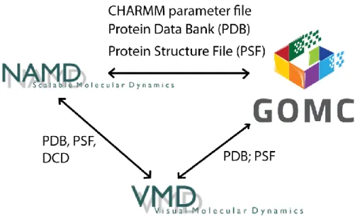
As an open source software engine, GOMC is designed to use standardized input and output file formats, allowing users to work seamlessly between GOMC and other simulation engines such as NAMD [10], and analysis and visualization tools such as VMD [74]. Figure 19 shows the compatibility between GOMC, NAMD, and VMD.

Figure 19: GOMC I/O compatibility with file formats used by other simulation engines

For input, the Protein Structure File (PSF) [75] format describes the structure of the system molecules, such as the bonds, angles, and dihedrals that make up each molecule. Protein Data Bank (PDB) [76] file formats are used to describe the 3D structure of molecules, such as the par-ticles of the molecules and the coordinates of those parpar-ticles. Application-specific file types are used to specify simulation parameters such as temperature, volume, and number of steps.

3.1.4 Initialization

Molecules’ coordinates, angles, dihedrals, random number generators, and system parameters are initialized at the start of the simulation. The coordinates are initialized by reading the PDB, while the PSF files are used to initialize the structure of each molecule, including the angles and dihedrals.

System parameters are read from the input configuration file. The configuration file specifies most of the system variables such as initial box dimensions, move percentages, number of simula-tion steps, input and output file names, output frequency, temperature, cutoff distance, and ran-dom number seed specification.

3.1.5 Random Number Generation

Random numbers have an essential role in the MC method. Random numbers are used to se-lect moves and determine the acceptance of them. There are many algorithms to generate uniform pseudorandom numbers. GOMC uses Mersenne Twister algorithm to generate the different ran-dom sequences used in GOMC. Mersenne Twister is one of the most commonly used pseudoran-dom number generators due to its long period (219937 – 1), fast random number generation, and its statistical randomness [33].

In the GPU version of GOMC, the random numbers are also generated on the CPU. When calling functions on the GPU, the required random numbers are passed to the GPU as parameters. In addition, if the random numbers are generated and moved to the GPU, there will be overhead of tracking how many random numbers are used, then when that stream is consumed, the CPU must generate another sequence and move it to the GPU. Although the cuRand package can be used to generate random numbers, this will not generate the same random stream of random numbers on both the serial and GPU versions of GOMC.

3.2 Main System Functionality

This section will focus on describing how energy calculations are done in GOMC and how different Monte Carlo ensembles work in GOMC.

3.2.1 Energy Interactions

Energy interactions are the main functions in the simulation, as they are a key factor in deter-mining the acceptance of moves. Energy interactions may involve all the system molecules, such as when calculating the system’s total energy, or a certain molecule interaction, or even a single