Semantic Segmentation and Completion of 2D and 3D Scenes

(1)

SEMANTIC

SEGMENTATION

AND

COMPLETION

OF

2D

AND

3D

SCENES

D

ISSERTATION

zur

Erlangung

des

Doktorgrades

(

Dr.

rer.

nat.

)

der

Mathematisch-Naturwissenschaftlichen

Fakultät

der

Rheinischen

Friedrich–Wilhelms–Universität,

Bonn

vorgelegtvon

M

ARTIN

G

ARBADE

aus

Saar

burg

(2)

(3)

Angefertigt mit Genehmigung der Mathematisch-Naturwissenschaftlichen Fakultät der Rheinischen Friedrich–Wilhelms–Universität Bonn

1. Gutachter / 1stAdvisor: Prof. Dr. Juergen Gall 2. Gutachter / 2ndAdvisor: Prof. Dr. Simone Frintrop Tag der Promotion / Day of Promotion: 25.11.2019 Erscheinungsjahr / Year of Publication: 2019

(4)

(5)

v

Abstract

by Martin Garbade

for the degree of Doctor Rerum Naturalium

Semantic segmentation is one of the fundamental problems in computer vision. This thesis addresses various tasks, all related to the fine-grained,i.e.pixel-wise or voxel-wise, seman-tic understanding of a scene. In the recent years semanseman-tic segmentation by 2D convolutional neural networks has become as much as a default pre-processing step for many other com-puter vision tasks, since it outputs very rich spatially resolved feature maps and semantic labels that are useful for many higher level recognition tasks. In this thesis, we make sev-eral contributions to the field of semantic scene understanding using an image or a depth-measurement, recorded by different types of laser sensors, as input.

Firstly, we propose a new approach to 2D semantic segmentation of images. It consists of an adaptation of an existing approach for real time capability under constrained hardware demands that are required by a real life drone. The approach is based on a highly optimized implementation of random forests combined with a label propagation strategy.

Next, we shift our focus to what we believe is one of the important next forefronts in computer vision: To give machines the ability to anticipate and extrapolate beyond what is captured in a single frame by a camera or depth sensor. This anticipation capability is what allows humans to efficiently interact with their environment. The need for this ability is most prominently displayed in the behaviour of today’s autonomous cars. One of their shortcomings is that they only interpret the current sensor state, which prevents them from anticipating events which would require an adaptation of their driving policy. The result is a lot of sudden breaks and non-human-like driving behaviour, which can provoke accidents or negatively impact the traffic flow.

Therefore we first propose a task to spatially anticipate semantic labels outside the field of view of an image. The task is based on the Cityscapes dataset, where each image has been center cropped. The goal is to train an algorithm that predicts the semantic segmentation map in the area outside the cropped input region. Along with the task itself, we propose an efficient iterative approach based on 2D convolutional neural networks by designing a task adapted loss function.

Afterwards, we switch to the 3D domain. In three dimensions the goal shifts from as-signing pixel-wise labels towards the reconstruction of the full 3D scene using a grid of labeled voxels. Thereby one has to anticipate the semantics and geometry in the space that is occluded by the objects themselves from the viewpoint of an image or laser sensor. The task is known as 3D semantic scene completion and has recently caught a lot of attention. Here we propose two new approaches that advance the performance of existing 3D seman-tic scene completion baselines. The first one is a two stream approach where we leverage a multi-modal input consisting of images and Kinect depth measurements in an early fu-sion scheme. Moreover we propose a more memory efficient input embedding. The second

(6)

vi

approach to semantic scene completion leverages the power of the recently introduced gen-erative adversarial networks (GANs). Here we construct a network architecture that follows the GAN principles and uses a discriminator network as an additional regularizer in the 3D-CNN training. With our proposed approaches in semantic scene completion we achieve a new state-of-the-art performance on two benchmark datasets.

Finally we observe that one of the shortcomings in semantic scene completion is the lack of a realistic, large scale dataset. We therefore introduce the first real world dataset for semantic scene completion based on the KITTI odometry benchmark. By semanti-cally annotating alls scans of a 10 Hz Velodyne laser scanner, driving through urban and countryside areas, we obtain data that is valuable for many tasks including semantic scene completion. Along with the data we explore the performance of current semantic scene completion models as well as models for semantic point cloud segmentation and motion segmentation. The results show that there is still a lot of space for improvement for either tasks so our dataset is a valuable contribution for future research into these directions.

(7)

List of Figures

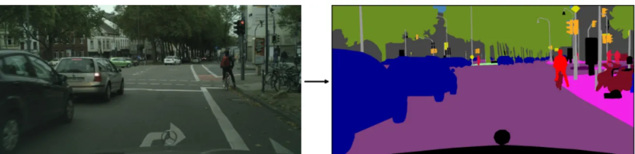
1.1 Example of an input and output pair for the task of semantic segmentation. Every

pixel of the input RGB image has to be assigned to a class label. . . 9

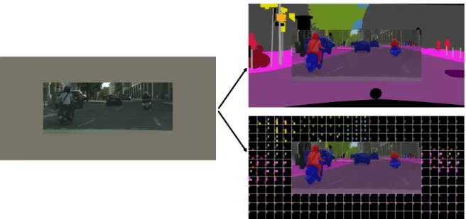
1.2 Visualization of input and output to the 2D spatial anticipation of semantic categories

task. We define two tasks. The first one (top right) requires to predict a pixel-wise semantic segmentation map in the grey area where no sensory input is given. The second task (bottom right) requires a cell wise prediction, where each cell contains a

boolean indicator, highlighting which classes are occurring in the respective cell. . . 10

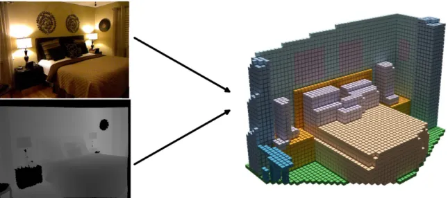
1.3 Visualization of input and output to the 3D semantic scene completion task. Top left:

Input RGB image. Bottom left: Input depth map. Right: Target - a voxelized and

semantically labeled representation of the 3D scene. . . 11

2.1 Milestones of CNN-architecture development. Top: LeNet-5 (LeCun et al., 1998),

Middle: AlexNet (Krizhevsky et al., 2012). Bottom: Comparison of VGG-19

Si-monyan and Zisserman(2015) and ResNet (He et al., 2016). . . 18

2.2 Skip-Connection mechanism as proposed by (He et al., 2016). . . 20

2.3 Dilated convolution proposed byChen et al.(2015). Input resolution is7ˆ7(bottom)

and the output resolution3ˆ3(top). The output resolution can be increased to the

same level as the input by adding a 0 padding to the input layer of half the kernel size. 21

2.4 Visualization of a2ˆ2strided deconvolution with kernel size3ˆ3, input resolution

is2ˆ2(bottom), input resolution is5ˆ5(top). In order to perform the deconvolution

an automatic 0-padding is being added to the input, depending on the kernel size k,

the size of the padding ispk`1q{2. . . 22

2.5 Architecture of the DCGAN proposed by (Radford et al., 2015). Both the generator

and the discriminator are fully convolutional neural networks. While the generators generates images from a randomly sampled input vector, the discriminator classifies whether the input image he got was real (sampled from the ground truth) or fake

(generated by the generator). Image adapted fromRadford et al.(2015). . . 23

4.1 For efficient segmentation, we use a quadtree to create superpixels and classify the

superpixels by a random forests. . . 36

4.2 Accuracy and average prediction time with respect to the number of trees. . . 40

4.3 Accuracy and average prediction time for one tree using different quadtree depths

when creating superpixels. The results are reported forsp-fr-Gauss2. . . 41

4.4 Examples of segmentation results. First row: original image. Second row: pixel

stride 1. Third row:sp-fr. Fourth row: sp-fr-Gauss2 + propagate. Fifth row: sp-fr-Gauss2 + sm. + prop. Sixth row: ground truth. . . 43

5.1 Training procedure for SASNet. The SASNet is trained on crops of masked images.

The mask marks the visible (Ω1) and the invisible regions (Ω2). A detailed

(12)

vi List of Figures

5.2 TheF1score is computed for cells outside the visible region and measures if for each

cell the same labels are predicted (right) as they occur in the ground-truth

segmenta-tion map (left). . . 49

5.3 Qualitative results for the pixel-wise label prediction using L1 loss. The first row

shows an RGB image and the inferred semantic segmentation using the approach of Chen et al. (2015). The second row shows the result for color-SASNet (left), which uses the RGB image of the first row as input, and for label-SASNet (right), which uses the inferred labels as input. The inner white rectangle marks the boundary

between observed and unobserved regionsΩ1andΩ2. The label-SASNet anticipates

the semantic labels inΩ2better than color-SASNet. The last row shows the result of

label-SASNet if the prediction is performed in two (left) or three steps (right). The additional white rectangles mark the growing regions that are predicted in each step.

Compared to the second row, the labels are better anticipated at the border. . . 50

6.1 Using the protocol of Song et al. (2017), ground truth labels are provided for all

voxels of a 3D volume. Voxels that are outside the intersection of the camera frustum and ground truth volume are outside the room or outside the view and not taken into account. Within the intersection, there are observed surface voxels (green) and observed non-occupied voxels (light gray), but other voxels are not observed by the

camera. These voxels are either non-occupied (blue) or belong to an object (black). . 57

6.2 a) The proposed two stream approach for semantic scene completion transforms first

the depth data and RGB image into a volumetric representation, which represents the geometry and semantic of the visible scene and then uses a 3D-CNN to infer a 3D semantic tensor for the entire scene. b) Given 2D depth map and camera pose, a binary voxel mask is created by setting each voxel that belongs to a depth pixel to one and all other voxels to zero (blue). c) Visualization of TSDF vs. flipped TSDF. One can see the long ‘shadow’ caused by the observed surface which produces high gradients at the occlusion boundary (between -1 and 1). In the flipped TSDF, this

effect is suppressed. The gradient is highest at the surface. . . 57

6.3 Architecture of the 3D-CNN. The parameters of the convolution kernels are denoted

as (number of filters, kernel size, stride, dilation). All but the last convolution layer

have a ReLU activation function assigned to it. Arrows indicate skip connectionsHe

et al. (2016) where the output of one convolution layer is added to another output at a later stage. Pool denotes max pooling. The output is a volume that is 4 fold downsampled with respect to the input of the 3D CNN and encodes for every voxel

the probability of it being empty (label 0) or to belong to one ofKsemantic classes. 59

6.4 Qualitative results on NYUv2 Kinect. From left to right: Input RGB-D image,

ground truth, result obtained by Song et al. (2017), and result obtained by our

ap-proach. Overall, our completed semantic 3D scenes are less cluttered and show a

(13)

List of Figures vii

7.1 Proposed network architecture. The generator network takes a depth image as input and predicts a 3D volume. The discriminator network takes either the generated 3D volume or the ground truth volume as input, then classifies them as real or fake. The parameters of each layer are shown as (number of filters, kernel size, stride) in the case of convolutions and as (number of output channels) in the case of fully

connected layers. . . 69

7.2 Qualitative results on NYU CAD. The first three columns show the input depth image with its corresponding color image, ground truth volume, and the results

ob-tained bySong et al.(2017). The fourth and fifth columns show the results obtained

by our approaches. . . 73

7.3 Comparison of the loss behaviour of the discriminator networks. . . 74

8.1 Our dataset provides dense annotations for each scan of all sequences from the KITTI

Odometry Benchmark (Geiger et al., 2012). Here, we show multiple scans

aggre-gated using pose information estimated by a SLAM approach. See also the video to

get a better impression of the consistency and quality of the provided annotation. . . 76

8.2 (Top) Single scan and (Bottom) multiple superimposed scans with labels. Also

shown is a moving car in the center of the image resulting in a trace of points. . . 79

8.3 Label distribution. Number of labeled points per class. Also shown are the root

categories for the classes. For movable classes, we also show the number of points

on non-moving (solid bars) and moving objects (hatched bars). . . 80

8.4 IoU vs. distance to the sensor. . . 84

8.5 Examples of inference for all methods. The point clouds were projected to 2D using

a spherical projection to make the comparison easier. . . 85

8.6 Example of using sequence information from SLAM poses to aggregate history. Top:

Original scan projected to a64 ˆ900image. Middle: Same scan projected to a

128ˆ900image. The image becomes sparse because the laser scanner only has64

beams. Bottom: Result of aggregating the last 5 scans using the SLAM poses and

projecting into to128ˆ900resolution. Projection becomes densely populated again. 88

8.7 Left: Visualization of the incomplete input for the semantic scene completion

bench-mark. Note that here we also show the labels for better visualization. However, the real input is a single raw laser scan without any labels. Right: Corresponding target

output representing the completed and fully labeled 3D scene. . . 89

8.8 Point cloud labeling tool. In the upper left corner the user sees the tile and the sensor’s

path indicated by the red trajectory. . . 91

(14)

(15)

List of Tables

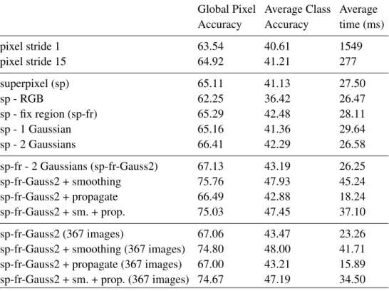
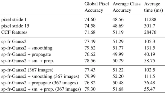
4.1 Results for one tree trained on all 468 training images. The last 4 rows report the

results when only the sequences recorded with 30 Hz are used for training (367). . . 38

4.2 Results for 10 trees trained on all 468 training images. The last 4 rows report the

results when only the sequences recorded with 30 Hz are used for training (367). . . 40

4.3 Comparison with state-of-the-art approaches. The first six rows shows results for

all 468 training images. The lower part report the results when only the sequences

recorded with 30 Hz are used for training (367). . . 42

5.1 Quantitative results for spatial anticipation on the Cityscapes dataset (Cordts et al.,

2016). RGB or Label denote if color-SASNet or label-SASNet are used. L₁ stands

for pixel-wise loss andL2for the cell-wise loss.kis the kernel size and stride used to

compute theL2 loss during training. The third column indicates if the SASNet was

applied gradually using 2, 3 or 4 steps. The fifth column is the pixel-wise evaluation

using%IoU. The other columns are F1 scores expressed in%computed for the

cell-wise evaluation. The size of the cells is specified as c. The last line shows the result

for a simple border replication. . . 52

6.1 Impact of the quality of the semantic input. For the version ‘RGB image’, the

2D-CNN is omitted and the color values of the pixels instead of the semantic information

is stored in the semantic volume. . . 61

6.2 2D semantic segmentation accuracies on the NYUv2 dataset (%IoU). In both cases,

a CRF is used. . . 61

6.3 Impact of the number of channels for the semantic volume. 12 channels refers to

one-hot encoding. . . 62

6.4 Impact of the input for the 3D-CNN. The proposed architecture is shown in

Fig-ure 6.2 a). The versions ‘with fTSDF’ refers to a version where not only the semantic

volume but also the flipped TSDF volumeSong et al.(2017) are used. . . 62

6.5 Comparison to the state-of-the-art. . . 63

7.1 Comparison of models for semantic scene completion results on the NYU Kinect.*

denotes that the network is trained on SUNCG and fine-tuned on NYU. . . 72

7.2 Comparison of models for semantic scene completion on the NYU CAD (Firman

et al., 2016). *denotes that the network is trained on SUNCG and fine-tuned on NYU. 72

7.3 Comparison with the state-of-the-art networks on the SUNCG . . . 73

8.1 Overview of other point cloud datasets with semantic annotations. Ours is by far the

largest dataset with sequential information. 1Number of scans for train and test set,

2_{Number of points is given in millions,}3_{Number of classes used for evaluation and}

number of classes annotated in brackets. . . 77

8.2 Single scan results (19 classes) for all baselines on sequences 11 to 21 (test set). All

(16)

x List of Tables

8.3 Approach statistics. . . 84

8.4 Single scan vs. multiple scan results. . . 86

8.5 IoU results using a sequence of multiple past scans (in %). Shaded cells correspond

to the IoU of the moving classes, while unshaded entries are the non-moving classes. 87

8.6 IoU results using a sequence of multiple past scans (in %). . . 87

8.7 Results for scene completion and class-wise results for semantic scene completion

(in %). . . 90

8.8 Approach statistics. ˚ in number of epochs means that it was started from the

pre-trained weights of the single scan version. . . 93

(17)

Nomenclature

Abbreviations

An alphabetically sorted list of abbreviations used in the thesis:

AI Artificial Intelligence

BOW Bag of words

CAD Computer-aided design

CRF Conditional random field

CNN Convolutional Neural Network

DCNN Deep Convolutional Neural Network

DNN Deep Neural Network

EM Expectation Maximization

GAN Generative Adversarial Network

HOG Histogram of Oriented Gradients

IoU Intersection over Union

m meters

MAP Maximum-a-Posteriori

MRF Markov random field

RGB-D RGB-Depth

SGD Stochastic gradient descent

SIFT Scale invariant feature transform

SLAM Simultaneous localization and mapping

SVM Support vector machine

Frequently Used Symbols

I Image G GraphG “ tV,Eu V Vertices of graphG E Edges of graphG E Energy function L Loss function p Probability φp¨q Unary potential ψp¨,¨q Pairwise potential θ Parameters

(18)

(19)

List of Publications

• Real-time Semantic Segmentation with Label Propagation

Rasha Sheikh, Martin Garbade, and Juergen Gall

In ECCV Workshop on Computer Vision for Road Scene Understanding and Autonomous Driving (CVRSUAD), 2016

https://pages.iai.uni-bonn.de/gall_juergen/download/jgall_ realtimesegmentation_cvrsuad16.pdf

• Thinking Outside the Box: Spatial Anticipation of Semantic Categories

Martin Garbade, and Juergen Gall

In British Machine Vision Conference (BMVC), 2017.

https://pages.iai.uni-bonn.de/gall_juergen/download/jgall_ spatialanticipation_bmvc17.pdf

• Two Stream 3D Semantic Scene Completion

Martin Garbade, Yueh-Tung Chen, Johann Sawatzky, and Juergen Gall

In CVPR Workshop on Multimodal Learning and Applications Workshop (MULA), 2019. https://arxiv.org/abs/1804.03550

• 3D Semantic Scene Completion From a Single Depth Image using Adversarial Training

Yueh-Tung Chen, Martin Garbade, and Juergen Gall

In IEEE International Conference on Image Processing (ICIP), 2019. https://arxiv.org/abs/1905.06231

• A Dataset for Semantic Segmentation of Point Cloud Sequences

Jens Behley *, Martin Garbade *, Andres Miloto, Jan Quenzel, Sven Behnke, Cyrill Stachniss, and Juergen Gall

In IEEE International Conference on Computer Vision (ICCV), 2019. https://arxiv.org/pdf/1904.01416.pdf

(20)

(21)

»What is good?« Ye ask.

To teach a machine how to see is good.

(22)

(23)

Acknowledgements

Having finished writing my thesis and now sitting in a hotel in Long Beach - Los Angeles - where I just got to attend what was arguably the largest computer vision conference in the history of the field (CVPR’19), it feels like a good moment to look back.

I had a great time during my PhD and the luxury of studying one of the most vibrant and fastest growing research fields of today and thereby being accompanied by some of the most proficient people. I’d like to thank them here!

First of all, I want to thank Prof. Jürgen Gall for accepting me as his PhD student. Having graduated in physics, this was a huge opportunity for me and required a lot of trust from his side. Working with Jürgen has been very efficient and uncomplicated. He was always there for questions and helped with many good ideas. Especially before deadlines, when many papers had to be edited often until late into the night, he helped us getting the job done without batting an eye.

Besides I’d like to thank Prof. Simone Frintrop, Prof. Thomas Schultz and Prof. Stefan Linden for accepting to be part of my PhD evaluation committee.

Next I’d like to thank my working group who made this PhD a memorable time with entertaining conversations and prolific discussions about research. First I’d like to thank Johann Sawatzky with whom I had by far the most frequent and deepest discussions (work- and non-work-related). Another thank goes to my former office mates Umar Iqbal and Mohsen Fayyaz whom I saw more often than anyone in my life at the time, and who always guaranteed for a nice and friendly working environment. A special thanks goes to Alexander Richard, who often gave me good advice and also fueled the efficiency of the entire group by his nice scheduling tool. Next I’d like to thank Hildegard Kühne, Ahsan Iqbal, Sovan Biswas, Andreas Döering, Yasser Souri, Julian Tanke, Rania Briq and Yazan Abu Farha for being such good colleagues that were all very open, friendly and helpful to me. Another big thank goes to Jens Behley, a long-time computer vision companion, whom I had the honor of collaborating with in the final project of my PhD as well as to Rasha Sheikh for smoothly handing over the MoD project to me. Last but not least, I’d like to thank our current and former master students, namely Christian Grund for being a very prolific Hiwi and a crack in Blender visualizations, Yueh-Tung, whom I was happy to supervise during his master thesis and Anna Kukleva, for discussions and being a fun travel mate at the CVPR.

Schließlich möchte ich mich bei meiner Familie und Geschwistern bedanken, die mir bei allem immer zur Seite gestanden haben und die mit mir gemeinsam durch etliche Deadlines gefiebert haben. Darüberhinaus danke ich allen meinen Freunden, die während der gesamten Zeit für die notwendige und erholsame Ablenkung gesorgt haben.

(24)

(25)

C

HAPTER

1

Introduction

Contents

1.1 Motivation . . . 5

1.1.1 Why Computer Vision? . . . 5

1.1.2 Applications of Computer Vision . . . 6

1.1.3 History of Computer Vision . . . 7

1.1.4 Why Semantic Segmentation? . . . 7

1.1.5 Open Problems in Semantic Segmentation . . . 8

1.2 Problem Formulations . . . 9

1.2.1 Semantic Segmentation . . . 9

1.2.2 Spatial Semantic Anticipation . . . 10

1.3 Contributions . . . 12

1.4 Thesis Structure . . . 13

1.1

Motivation

1.1.1 Why Computer Vision?

One of the greatest achievements that humans might solve within our lifetime is construction of intelligent, autonomous robots. The vision already caught Hollywood’s attention, although mostly in a negative way. Movies like ‘Terminator’ or ‘The Matrix’ describe the future as a war between intelligent machines and humans. We, on the contrary, will focus on the potential for good that lies in this technology.

Along with the discovery of electricity and inventions like the steam engine and computers, the invention of autonomous robots is another milestone in the people’s pursuit to replace harsh, dangerous, and costly human labour by machines. It will be interesting to see, if we are the generation to witness armies of robots, harvesting crops, farming land or perhaps even build entire cities at the command of a single person. They could be used to rebuild cities destroyed by war or to restore precious architectural artifacts like Notre-Dame of Paris which recently burned almost to the ground. At least in case of Notre-Dame, 3D reconstruction with the help of computer vision techniques is already likely to play a role in its restoration.

Just as the invention of engines and electricity helped to replace the human muscle by machines, the goal of computer vision and its close relative artificial intelligence are bound to replace the human eyes and brain. At the end of the day, all a man will need is a will and a machine to execute it. In a society equipped with fully autonomous machines, most of the dangerous, laborious and undesired

(26)

6 Contents

jobs might be done by machines. Even so much so that mainly creative, social and managing jobs might be left, a vision that scares some people rather than it entertains them. However, history teaches us, that people are very creative when it comes to inventing new jobs, which are likely to be more comfortable than those taken over by machines.

The question is, why aren’t we already there? After all, we are able to construct robots in all shapes and forms. The reason is that one final wall on our way there has not been conquered yet: Perception. Though we are able to build robots and manually control them, the goal must be that they interact autonomously with their environment such that all they need is a high level plan and they themselves will figure out how to execute it in detail. This is the motivation for doing computer vision. The goal is to teach machines to see the world, similar to how we humans see it. Thus they can effectively interact with it, navigate through it, make predictions about its state, grasp things and put them somewhere else, mow lawn, harvest crops or drive anyone safely from A to B. This thesis is dedicated to one of the most important technological goals in society today: Bringing perception to machines.

1.1.2 Applications of Computer Vision

Beyond the big dreams, computer vision has been an active field of research for the past 6 decades. It already has reached some impressive goals. We are already surrounded by cleaning robots or cars equipped with computer vision systems to increase the safety.

Since May 2012 Google followed by other companies like Uber and Tesla are already driving with fully autonomous cars through cities of the United States. These cars still have a human pilot that can take over the driving in case the system fails, but the amount of kilometers driven without human interference increases steadily. The chase for the first fully autonomous cars has attracted peoples attention and sparked their ambition in a truly Olympic spirit.

Though many of the first autonomous cars were equipped with a variety of sensors (radars, ultra sound, Velodyne-laser-range scanners), currently most mass produced vehicles with computer vision techniques involve a camera sensor. The advantage over the above mentioned sensors is clear. A

camera is extremely cheap („1 Eur vs„60 000 Eur for a Velodyne Laser currently) and has the

richest signal of all due to its storage of RGB information and it has by far the best resolution in the far field. On a camera picture one can easily identify objects in a distance of up to 200m whereas a laser range signal becomes rather uninterpretable after 50m distance. On the other hand, RGB images are much harder to interpret and thus machine learning systems become potentially more error prone as the variance in the data increases. In 2017 a Tesla car, equipped with a vision based driving assistant mistook a white truck for the class ‘sky’ which made the inattentive driver the first

victim of a computer vision controlled car1.

All of the before-mentioned sensors only measure some distance value to an obstacle which is good for collision avoidance, however often crucial parts of the scene, like the difference between sidewalk and road only become obvious in a picture, which has color values. This thesis, therefore, deals with the ‘king of the sensors’, the RGB camera.

(27)

1.1. Motivation 7

1.1.3 History of Computer Vision

Computer vision is an extremely fast advancing field and in many ways fields like the Wild West among the sciences. Today state-of-the-art algorithms are usually ‘dethroned’ after not much more than half a year. The community is open in sharing data and models, so people can immediately start from a state-of-the-art algorithm and improve on it. The usage of common benchmark datasets and evaluation protocols ensures the fair comparison between algorithms. During my PhD a seismic shift shook the entire research community: The successful rise of deep learning techniques above all previous, sophisticated and highly engineered methods. Since then, the chase for better models was partly overshadowed by a chase for more annotated data.

In the early 60s computer vision began as an engineering problem. Datasets were extremely simple and people tried to come up with domain specific expert knowledge in order to recognize objects in images. Apart from these early approaches the field was for the most time of its existence ruled by the following paradigm: Engineer hand-crafted features that capture the important aspects of the object you want to detect, then apply some intermediary processing to either quantize the features or to aggregate them, finally use a classifier to determine which of the predefined classes you have detected.

This paradigm shifted entirely after in 2012 the most successful approach winning the ImageNet

image recognition challenge used an entirely different approach: Deep learning2.

The concepts of deep learning were old. Already in the sixties people tried to emulate the learning

behaviour of the human brain by an algorithm3. This was the beginning of a new research field called

artificial intelligence (AI). Though people believed in the power of AI for some years, the algorithms

were lacking far behind other more engineered approaches. This lead to an era called AI winter4,

where the hype around AI burst like a bubble and high ranking conferences refused to accept papers that claimed new advances in the field.

Luckily a small group of people clang on to the idea, such that over 4 decades later, when com-puters had much more parallel computing power due to GPUs and the amount of annotated data was orders of magnitudes larger, they could outperform all existing approaches with a simple end-to-end system not much unlike one used in the 70s which could only recognize numbers between 0 and 9

on 28ˆ28 pixel images.

1.1.4 Why Semantic Segmentation?

After this short detour into the history of computer vision, we will now explain why we focus on semantic segmentation and its related fields. Compared to one of the oldest computer vision tasks (image classification), semantic segmentation is something like a ‘next step’. Since image classifica-tion has made tremendous advances, the interest in the field declines. As people see it as ‘solved’ or rely on non-academic research with their greater access to data and computational resources. Instead people come up with new and more challenging problems. Compared to image classification, seman-tic segmentation is the next harder step, though being still very basic in its goal: Assign a class label to every pixel in an image. By trying to label every pixel the problem becomes harder, as one has to deal with localization of objects, identifying their shape, boundaries between objects as well as very

2

https://qz.com/1307091/the-inside-story-of-how-ai-got-good-enough-to-dominate-silicon-valley/

3

https://towardsdatascience.com/rosenblatts-perceptron-the-very-first-neural-network-37a3ec09038a

(28)

8 Contents

small objects that only cover a minuscule part of the image and often need context information in order to be classified.

Again a traditional approach would use a bottom-up graph based segmentation algorithm to com-pute superpixels, then use an object classifier on these superpixels and occasionally a conditional random field (CRF) in a post-processing step to enforce more label consistence in the local neigh-bourhood of pixels.

Today, virtually all state-of-the-art approaches rely on fully convolutional neural networks, which are extremely powerful and flexible. There is no need for hand-crafting features anymore and almost any parameter of the model itself is learned during the training of the network so the need for tuning hyperparameters is minimal. Furthermore the same CNN architecture can be used for almost any computer vision related problem with some slight domain specific adaptation. CRFs are still used in some modern approaches to refine the segmentation results.

1.1.5 Open Problems in Semantic Segmentation

Similar to image recognition, semantic segmentation has made impressive advances in a couple of years, so much that even in this field people start moving away in the search for harder problems to be solved. On the other hand, fully convolutional CNNs pre-trained for semantic segmentation have become ubiquitous as feature extractor and starting point for almost any algorithm of related fields (pose estimation, action recognition, tracking, monocular depth estimation).

In this thesis we follow the same pattern. Our first approach which does classical semantic segmentation stems from a time, when the entire field was transitioning towards CNN based methods. It is a classic approach which is highly optimized to achieve real-time capabilities on a GPU-free hardware device (drone). This approach is effective as our experiments show, though it is likely that future drones will carry small GPUs in case the power consumption is not to high as compared to CPUs.

After that we asked ourselves, what could be the next frontier in computer vision / semantic scene understanding. One hint comes from the observation of autonomous cars: Apart from some famous stories that made it to the news of fatal failure of computer vision algorithms: 1) Man crashes his Tesla into a white truck, since the image recognition system mistakes the white truck for "sky" (probably due to greyscale images as used by Mobileye having less color contrast) or 2) Car drives over (seemingly drunken) person that crosses the road, pushing a bike while ignoring the giant Uber SUV approaching him, again with fatal consequences. These accidents hint to the fact that current systems are likely to perform reliably 99.9% of the time, but fail utterly in the occurrence of rare events which are not part of the training data. The above listed examples are shocking as they are easy to manage by a human driver

The latter story could be already related to our problem. The key observation comes from sim-ple observation of the driving performance of current autonomous cars. It looks, like their driving behaviour is very non-human-like, meaning they drive extremely cautiously, stop at every hard inter-pretable situation and most importantly seem not to understand how the scene surrounding them will evolve in the near future.

This is a new task we address with this thesis: The problem of anticipation. Humans automati-cally can infer a lot of information in a top down process. They know from experience a lot about the scene, objects in it and their likely behaviour.

(29)

1.2. Problem Formulations 9

Figure 1.1: Example of an input and output pair for the task of semantic segmentation. Every pixel of the input RGB image has to be assigned to a class label.

There are two types of anticipation that are of interest: Temporal anticipation and spatial antici-pation. Temporal anticipation would deal with the dynamic of a given scene in the near future. This is a topic closely related to action recognition which lies outside the focus of this thesis. The other type of anticipation is spatial anticipation. This means given an input image we try to extrapolate the scene to parts that are outside the field of view of a sensor or otherwise occluded. This is the exact part that we focus on in this work. First we start in two dimensions. We ask ourselves: Given a 2D input image of a scene, what is the most likely semantic extrapolation of the scene beyond the image boundary. Thereby we effectively try to anticipate a scene and objects that are not yet visible but likely to occur. This might for example cause an autonomous car to drive safely as it anticipates pedestrians or playing children suddenly emerging from within a row of tightly parked cars. Just as humans learn to drive carefully in such situations as they anticipate the sudden occurrence of a person from experience, likewise we train a system that learns to anticipate similar events from data. Next we extend the idea to the 3D domain. The reconstruction of a 3D scene from a single input

image or depth measurement (e.g.by a Kinect or Velodyne laser sensor) has naturally to deal with

uncertainties due to sensor occlusions. From every element that composes the 3D scene only the surface that is visible to the sensor is detected. The backside of every element is occluded by the objects themselves. Humans however are able to predict the geometry and semantics of objects even in the occluded space. The field of 3D semantic scene completion tries to emulate this capability. In this thesis we present two new efficient approaches for the task of 3D semantic scene completion as well as a new benchmark suited to boost future research in the field.

1.2

Problem Formulations

We will now clarify for every task, addressed in this thesis, what is the exact input to each algorithm and the respective output.

1.2.1 Semantic Segmentation

Semantic segmentation is the task of assigning a semantic class label to every pixel of a 2D repre-sentation of a scene. Thereby elements composing the scene are simultaneously identified, localized and their shape delineated. Therefore the output looks like a map of semantic segments that belong to different class labels. Figure 1.1 shows an example.

(30)

10 Contents

Figure 1.2: Visualization of input and output to the 2D spatial anticipation of semantic categories task. We define two tasks. The first one (top right) requires to predict a pixel-wise semantic segmen-tation map in the grey area where no sensory input is given. The second task (bottom right) requires a cell wise prediction, where each cell contains a boolean indicator, highlighting which classes are occurring in the respective cell.

Assigning semantic meaning to the world as it is perceived is what a child learns while growing up. Thereby it develops a language which allows it to identify different objects as well as to com-municate and consciously reason about objects, matter, etc. and their relation to one-another and to itself. Thereby one has to take into account that words charged with a semantic meaning may stand in intricate relation to one another: Words like object, vegetation, wood, tree for example are in a hierarchical relationship where one word is either an abstraction of the other or includes it as an element of which composes another element. In the definition of today’s semantic segmentation benchmarks these hierarchical relations have to be taken into account. Most benchmarks propose a fixed list of predefined semantic class labels that are clearly distinguishable for a human annotator and do not have any semantic overlap with each other. In this thesis, we follow this pattern and only deal with datasets that provide non-hierarchical and unambiguous label categories.

All future tasks that involve interpreting image content enabling an autonomous robot to perceive its environment and to efficiently interact with it will either implicitly or explicitly have to solve the task of semantic segmentation.

1.2.2 Spatial Semantic Anticipation

Another major concept we deal with in this thesis is the task of spatial semantic anticipation. This task is defined as the prediction of semantic categories outside the field of view, i.e. without any sensory input data. In practice we take as input a 2D image of a scene. An example is shown in Figure 1.2. As output we generate a semantic segmentation map for the region surrounding the field of view, captured by the image. The thereby inferred semantic segmentation map is what we call “spatially anticipated”. It is an extrapolation of the scene as seen by the camera sensor. The

(31)

1.2. Problem Formulations 11

Figure 1.3: Visualization of input and output to the 3D semantic scene completion task. Top left: Input RGB image. Bottom left: Input depth map. Right: Target - a voxelized and semantically labeled representation of the 3D scene.

fundamental idea behind this task is that humans also extrapolate the surroundings of a scene given a single view. Even though the prediction might be ambiguous (since what is a valid extrapolation into the unseen part of a scene is inherently non-deterministic) making plausible predictions of a scene helps to efficiently navigate through it and to come up with an efficient path planning strategy. It also could prevent a robot from the need of exhaustively exploring an entire scene. Moreover, potentially dangerous events can be prevented. Without anticipation capabilities a ride in an autonomous car can be an unintuitive experience. This could lead to unexpected breaks or extreme driving manoeuvres, for example if a small child, initially occluded by cars parking along the edge of the road, suddenly runs onto the road. The probability of such events has to be estimated and the driving policy adapted accordingly.

1.2.3 Semantic Scene Completion

A natural extension of spatial 2D semantic label anticipation into the realm of 3D scene understand-ing is called 3D scene completion. In this task the input is some kind of sensory input, e.g. from a RGB-D camera or a RGB camera triggered by a Velodyne laser scanner mounted on a car. These sensors only capture appearance and geometric information from surfaces visible to the position of the sensor. As output however we generate a semantically labeled 3D voxel grid including those parts of the scene which are occluded by the visible surfaces. See Figure 1.3 for an example. E.g. if the camera captures the front and top of a bed or table, the output should contain a complete vox-elized version of this bed or table. Therefore, like in the 2D case, the algorithm has to anticipate the geometry and semantics of parts of the scene that are beyond what is recorded by the sensors. The motivation for this task is the same as for 2D spatial anticipation of semantic categories. In the 3D case however the geometry and proportionate object part sizes of the scene have to be reproduced as well.

(32)

12 Contents

1.3

Contributions

In this work we try to advance the field of semantic scene understanding on several fronts: On the one hand we provide 2 works in the field of 2D semantic image segmentation.

• The first work is a 2D semantic segmentation algorithm with real time performance and com-petitive accuracy tailored to run on a single threaded device. The idea came from a research project, the goal of which was to equip a research drone (also called “Unmanned Aerial Vehi-cle” - UAV) with on-device semantic segmentation capability to enable autonomous flight even in case of lacking contact to a ground station server. We propose a new method which is based on texton features and random forests and leverages quad-tree based label propagation as well as spatial Gaussians to achieve a competitive semantic segmentation accuracy while operating

in real time („ 30ms) on a single threaded CPU. We further provide an extensive study on

feature and parameter design choices and their impact on computation time and accuracy. • The second work is a seminal work in 2D spatial semantic label anticipation. To the best of

our knowledge we are the first to introduce this kind of task. We introduce two benchmarks based on the Cityscapes dataset. The first one measures how good a proposed extrapolation of a semantic segmentation matches with a pixel-wise segmentation map annotated by humans which we consider as ground truth. The second benchmark relaxes for the need of exact pixel-wise prediction in favour of a cell-pixel-wise prediction. In this case the area to predict is cut up into a grid of larger cells. All labels occurring in the pixel-wise annotated ground-truth are counted in a boolean histogram as being present or not present. The goal in this task is to predict the histogram for every cell. In contrast to the pixel-wise accuracy metric, the cell-wise prediction metric puts a less-hard constraint of the exact localization of a pixel which is inherently non-deterministic in the case of scene extrapolation and therefore allows for more practical predictions. Furthermore we propose CNN based models and a new loss function designed to efficiently solve these new tasks.

On the other hand we provide contributions for the task of 3D semantic scene completion • First we propose a new model in the recently emerged field of semantic scene completion

based on fully convolutional 3D-CNNs. We introduce a two stream architecture which fuses data from an RGB and a depth sensor to infer a 3D semantic completion of a scene. Further-more we show that inference time can be greatly improved while still achieving state-of-the-art performance.

• Secondly, we introduce an approach that examines the potential of generative adversarial net-works for the task of 3D semantic scene completion. Our best approach demonstrates that using conditional GANs can greatly improve the performance of 3D CNN architectures mod-elled for semantic scene completion. Furthermore, we identify that this performance is not robust across all evaluated benchmarks. Given that the concerned dataset is very small and has a high problem of misalignment between real world input data and synthetic annotated labels, we infer that there is a need for a new dataset in semantic scene completion.

• Lastly we introduce a new dataset suitable for 3D scene completion. As hitherto all 3D scene completion works either work on the very small NYUv2 benchmark or on synthetic data taken

(33)

1.4. Thesis Structure 13

from the SUNCG dataset, there is an ardent need for a new large scale dataset in order to ef-fectively train CNN architecture based models on this task. Along with the dataset we provide a quantitative evaluation of common 3D scene completion models on this new dataset. More-over, since the dataset consists of annotated laser scans from a point cloud dataset, we also explore the performance of current state-of-the-art semantic segmentation algorithms for point clouds as well as motion segmentation.

1.4

Thesis Structure

We begin by revising some theoretical concepts that underlay our models (Chapter 2). Then we give an overview of the related work (Chapter 3). Next, we present a work on 2D semantic segmentation (Chapter 4), followed by a work addressing the anticipation of semantic labels outside the field of view of a 2D image (Chapter 5). Afterwards, we change our focus to 3D where we first propose a new approach to 3D semantic scene completion based on a multi-modal input (Chapter 6) and secondly address the potential of generative adversarial networks in the context of 3D scene com-pletion (Chapter 7). Finally we introduce a new dataset that is the first large scale realistic dataset for 3D semantic scene completion and apart from that is suitable for many other tasks, like semantic segmentation on 3D point clouds (Chapter 8).

(34)

(35)

C

HAPTER

2

Preliminaries

We will now describe the most important models that our works are based on. We begin by dis-cussing random forests, a classifier, which is still of interest today in the context of devices with limited hardware. They allow for quick inference times even without parallel computing hardware like GPUs. Afterwards we focus on the major building block of nearly all computer vision related fields today: Convolutional neural networks (CNNs). Their dominance has only been established within the lifetime of this thesis and is still expanding. Another concept that is based on CNNs are generative adversarial networks (GANs), which also quickly gained popularity from their inception in 2014. One of our works explores the potential of GANs for the task of semantic scene completion. Finally we discuss the conditional random field (CRF), which is a graphical model defined on pixel class probabilities and is frequently used as a post processing step to increase segmentation accuracy throughout this thesis.

A random forest is a classifier consisting of an ensemble of binary decision trees. Though each indi-vidual tree by itself has a weak classification performance, the combination of several independently trained trees leads to a strong classifier. Random forests leverage the concept of stochastic discrim-ination to prevent overfitting to a specific training set. We now describe the concept and training procedure of random forests.

Criminisi and Shotton(2013) proposed a random forest for the task of semantic image

segmenta-tion. In their model each tree infers for an image pixelxthe class probabilityppc|x;θtqwherecis a

(36)

16 Contents

fashion by sampling from both the training data and the parameter space Θ. A robust estimator is

then obtained by averaging the predictors ppc|xq “ 1

T

ÿ

t

ppc|x;θtq, (2.1)

whereT is the number of trees in the forest. A segmentation of an image can then be obtained by

taking the class with highest probability for each pixel.

To learn the parameters θt of a tree t, first, pixels from the training data are sampled which

provide a set of training pairsS “ tpx, cqu. The tree is then constructed recursively, where at each

nodena weak classifier is learned by maximizing the information gain

θn“arg max θPΘ˜ $ & % HpSnq ´ ÿ iPt0,1u |Sn,i| |Sn| HpSn,iq , . -. (2.2)

WhileSndenotes the training data arriving at the noden,Θ˜ denotes the set of sampled parameters

and

HpSq “ ´ÿ

c

ppc;Sqlogppc;Sq

whereppc;Sqis the empirical class distribution in the setS. Each node becomes a weak classifier

fθpxqwith parametersθthat splitsSninto the two sets

Sn,i“ tpx, cq PSn:fθpxq “iu

with i P t0,1u. After the best weak classifier θn is determined,Sn,0 andSn,1 is forwarded to the

left or right child, respectively. The growing of the tree is terminated when a node becomes pure,

meaning it does only contain samples of a single class, orSnbecomes smaller than some threshold.

Finally, the empirical class distributionppc;S_lqis stored at each leaf nodel. During inference, one

can computeppc|x;θtqfor every pixelxand treetand infer the final class probability distribution

ppc|xqusing Equation 2.1.

2.2

Convolutional Neural Network (CNN)

A major building block of nearly all our models are convolutional neural networks (CNNs). We will briefly describe their history and neuroscientific motivation before explaining the architecture and functionality of a typical modern CNN.

2.2.1 History

Frank Rosenblatt, a psychologist and computer scientist, in 1958 published the ‘perceptron’ model

consisting of a single layer of neurons, randomly connected to the input (Rosenblatt, 1958). The

per-ceptron was implemented as a hard-wired machine without software using as input a grid of20ˆ20

photocells which were randomly wired to neurons while using electric motors for updating weights during learning. Nevertheless since the perceptron model consisted of a binary linear classifier it is considered the basis of today’s artificial neural networks.

(37)

2.2. Convolutional Neural Network (CNN) 17

The perceptron then developed into a multilayer perceptron (MLP) consisting of multiple layers

of perceptrons and capable of learning non-linear functions. Rumelhart et al. (1986) proposed the

backpropagation algorithm for training parameters of a multilayer-perceptron. LeCun et al.(1989)

applied backpropagation to a neural network recognizing digits in 2D images.

LeCun et al.(1998) introduced a convolutional neural network architecture, whose the basic func-tionality is similar to that of today’s architectures: The input was processed by a sequence operations consisting of convolutions, followed by the addition of a bias term, followed by a nonlinear transfor-mation (e.g. hyperbolic tangent or logistic function). The shift from sigmoid activation function to ReLU came due to the observation that sigmoid activations tend to saturate quickly and thus do not contribute to the learning anymore.

Though the field existed for a long time, high expectations and the consequent failure to achieve them, repeatedly led to phases of reduced interest into neural network based methods (phases called ‘AI winters’). The interest in the field was completely revived when Krizhevsky et al in 2012 fa-mously won the 2012 ImageNet challenge by a large margin. This success was mainly driven by two effects: The shift towards GPU based parallel processing and the availability of large scale datasets. This can be seen from the fact that the architecture of the Krizhevsky’s CNN strongly resembles

LeNet-5 byLeCun et al.(1998), apart from being significantly deeper.

2.2.2 Neuroscientific Background

The idea for the construction of a neural network was inspired by the study of the functionality of the human brain and perception. It is an attempt to emulate the process of visual perception by an algorithm. We briefly outline the concepts that influenced the conception of CNNs.

The human eye projects a 2D image of the outside world through a lens onto the retina. The retina consists of nerve cells which either register brightness or color. From the retina, the image is transferred via the optic nerve and the lateral geniculate nucleus (LGN) to the primary visual cortex (V1). Researchers have found that neurons in V1 perform operations resembling convolutions. V1 contains ‘simple cells’ which behave linearly with respect to a local neighborhood of the incoming receptive field and ‘complex cells’, which are invariant to spatial transformations of the input signal.

V1 also shows a 2D spatial structure like the retina,i.e.light shined onto different parts of the retina

only activate specific regions in V1. 2.2.3 Architectures

CNNs consist of a repetitive pattern of functional blocks. Each functional block processes an input by a sequence of operations to produce an output layer. The output layer is subsequently fed to another functional block. Figure 2.1 gives an overview over some historically influential CNN architectures. The most prominent architectural development, is that CNNs have become deeper over time. While LeNet (1980) only has two convolutional layers, AlexNet (2012) has 5, followed by VGG (2014) with 19 and ResNet (2016) with up to 100. As the networks become deeper, training becomes harder since the problem of ‘vanishing gradients’ increases.

Some design choices of the presented models are designate as useful and used in most modern architectures. AlexNet relied on Dropout to prevent overfitting, especially in the fully connected

layers. VGG, for example, restricted the spatial size of every convolution kernel to 3ˆ3, which

(38)

18 Contents Figur e 2.1 : Milestones of CNN-architecture de v elopment. T op: LeNet-5 ( LeCun et al. , 1998 ), Middle: Ale xNet ( Krizhe vsk y et al. , 2012 ). Bottom: Comparison of V GG-19 Simonyan and Zisserman (2015 ) and ResNet ( He et al. , 2016 ).

(39)

‘skip-connections’. AlexNet, VGG and ResNet all proved their efficiency by winning the ImageNet challenge (ILSVRC). Afterwards they were quickly adapted and applied in many related fields of computer vision.

For semantic segmentation the most important modification is the replacement of all fully

con-nected layers by a convolutional layer, as first proposed byLong et al.(2015). Thereby the last layer

becomes a pixel-wise classifier. These fully convolutional neural networks are extremely handy, as they are able to consume inputs and produce outputs of any size. In the following we will explain the behaviour of the individual components of CNNs as well as the training procedure.

2.2.4 Components

Convolutions

Convolutions are at the basis of the success of neural network based learning and image analysis. In contrast to fully connected layers they offer a significant reduction in the number of parameters

per layer through weight sharing,i.e.that the same kernel is applied to multiple regions of the input

feature. The convolution of a two-dimensional image I by a kernel K is defined by

Spi, jq “ pK˚Iqpi, jq “ ÿ m ÿ n Ipi´m, j´nqKpm, nq. (2.3)

In current CNNs the actual implementation of a convolution slightly deviates from this mathematical definition. First, to account for multiple channels of the input image or feature map, another dimen-sion is added to the kernel. Secondly, in contrast to Equation 2.3, the kernel K is flipped, which technically changes the convolution into a correlation, which is however irrelevant for the

function-ality of the CNN since the parameters of K are initialized randomly (Goodfellow et al., 2016). More

specifically, the computation of an elementZi,j,kof an output tensorZfrom an input tensorVwith

entriesVi,j,kwhere the indicesi, j, kdenote the channel, row and column dimension respectively, is

performed as follows: Zi,j,k is obtained by applying a convolution kernelK, then adding a biasb

followed by the transformation by some non-linear functionσ

Zi,j,k “σ ´ _ÿ l,m,n Vl,j`m,k`nKi,l,m,n`bi ¯ . (2.4)

where the non-linear function σis typically the ‘rectified linear unit’ (ReLU) introduced byGlorot

et al.(2011)

fpxq “maxp0, xq. (2.5)

Pooling

A pooling layer replaces every neuron of an input feature map by a summary statistic of its local

neighbourhood. A typical example is a 2ˆ2 max-pooling operation with stride 2. Thereby only

the maximum value of a rectangular 2ˆ2 region is copied to the output feature map, which is

(40)

20 Contents

Figure 2.2: Skip-Connection mechanism as proposed by (He et al., 2016).

The pooling operation has several motivations: Apart from reducing the memory consumption of subsequent layers, it also leads to an increase of the receptive field of subsequent convolutions. Moreover by integrating over the local neighbourhood information, the network becomes more robust to small translations of the input features.

Skip-Connection

A skip-connection allows information to flow unmodified from earlier layers to later layers in the network. Figure 2.2 illustrates the mechanism. The input to a convolutional block is forwarded

bypassing the block and added to its output layer.He et al.(2016) could show significant performance

improvements when adding the skip-connections to their CNN architecture. During the forward pass the skip-connections allow deeper layers to use information not only from previous but also from earlier layers. During the backward pass, the skip-connection allows gradients to flow unaltered to early layers, which helps to reduce the problem of vanishing gradients.

Batch-Normalization

A batch-normalization layer transforms every neuron to have approximately 0-meanµand a variance

σof 1, with respect to the training data. To achieve this a moving average of both values is computed

along the batch-dimension during the network training. During inferenceµandσare kept fix.

Batch-normalization has been introduced byIoffe and Szegedy(2015). They showed that

batch-normalization greatly speeds up the training time while at the same time making the training more robust towards the choice of hyperparameters like the learning rate or the initial values of the model parameters. However, batch-normalization can only be applied in cases, where the batch-size is larger than 1 and performs poorly for small batch-sizes.

Dilated Convolutions

Dilated convolutions is a concept that is quite frequently used in the domain of semantic segmenta-tion. They are convolutions with an increased kernel size but constant number of parameters. There-fore the learnable parameters are evenly placed on a regular grid and the non-occupied cells are filled up with zeros. These cells remain zero throughout the training. As one can see from Figure 2.3 this has the effect of increasing the receptive field without the need for decreasing the image resolution as in the case of pooling layers.

A strided convolution with strides, a kernelKwith elementsKi,j,k,lon an inputVproduces an

(41)

Figure 2.3: Dilated convolution proposed byChen et al.(2015). Input resolution is7ˆ7(bottom)

and the output resolution3ˆ3(top). The output resolution can be increased to the same level as the

input by adding a 0 padding to the input layer of half the kernel size. a

a_{Source: https://towardsdatascience.com/types-of-convolutions-in-deep-learning-717013397f4d} Zi,j,k “ ÿ l,m,n rVl,pj´1qˆs`m,pk´1qˆs`nKi,l,m,ns. (2.6) Deconvolutions

A frequently used method to increase the resolution of feature maps are deconvolutions. In contrast to convolutions they take as input a single neuron from the previous feature map, scalar multiply it with a convolutional kernel and add the result in the subsequent feature map. The process is repeated for all neurons in the input feature map and the results in the output feature map are aggregated via addition. Figure 2.4 shows an example of the process. There is an equivalent perspective of the same operation, which is what is actually implemented in most libraries. The aggregation of differently weighted kernels in the output layer is equivalent to a strided convolution, where the input feature map is first upsampled by placing the input on a higher resolution grid and setting all of the newly introduced cells to 0 and furthermore adding a 0-padding of half the kernel size at every border. The input is then convolved with the flipped version of the convolution kernel, hence the alternative name ’transpose-convolution’. Transpose convolutions and deconvolutions have different implementations, but yield identical results. Therefore, their names are used exchangeable.

2.2.5 Training

The training of a CNN is modelled as an optimization problem. The goal is to find the parameters

θ of a neural network that minimize a cost functionJpθq, which measures the performance of the

network on a training set of sizeN

Jpθq “

N ÿ

i“1

(42)

22 Contents

Figure 2.4: Visualization of a2ˆ2strided deconvolution with kernel size3ˆ3, input resolution is

2ˆ2(bottom), input resolution is5ˆ5(top). In order to perform the deconvolution an automatic

0-padding is being added to the input, depending on the kernel size k, the size of the padding is pk`1q{2.a

a

Source: https://towardsdatascience.com/types-of-convolutions-in-deep-learning-717013397f4d

whereLipx, yq is the loss function evaluated for a training sample i consisting of an input x and a

label y. The loss function measures the distance of the output prediction of the neural network to the label in a task specific metric. For classification tasks like semantic segmentation one typically uses a pixel-wise softmax cross-entropy loss

Li “ ´ ÿ cPC ˆ yiclog ¨ ˝ eyic ř c1_P_C eyic1 ˛ ‚ (2.8)

where yˆic is the class probability of the ground truth label of pixeli, which is1 for the true class

and0 otherwise. yic denotes the unnormalized predictions of the network for pixeli and classc.

In order to tune the initially randomly chosen parameters of the CNN, one applies backpropagation. During backpropagation one computes the gradient of every parameter in the network with respect

to the objective function J. Starting from the last layer fn, one can get the gradient of all earlier

layers fi by successive application of the chain rule, which for simplicity we show here for the

one-dimensional case Jpxq “fn˝ ¨ ¨ ¨ ˝f1pxq (2.9) BJpxq Bfi “ Bfn Bfn´1 ¨Bfn´1 Bfn´2 ¨. . .¨Bfi`1 Bfi . (2.10)

With the help of the gradient with respect to the weights∇WLon can update the trainable weights

such that they minimize the cost functionJ, for example via stochastic gradient descent (SGD):

W “W ´λ∇WL (2.11)

Stochastic refers to the fact that L is not computed for the entire training data at once but instead for a small randomly sampled batch of data, before updating the weights. In practice one uses more

(43)

2.3. Generative Adversarial Network 23

Figure 2.5: Architecture of the DCGAN proposed by (Radford et al., 2015). Both the generator and the discriminator are fully convolutional neural networks. While the generators generates images from a randomly sampled input vector, the discriminator classifies whether the input image he got was real (sampled from the ground truth) or fake (generated by the generator). Image adapted from

Radford et al.(2015).

refined variants of SGD such as SGD with momentum or ADAM which gather some additional

statistics of the gradients in order to accelerate the training. The learning rateλis one of the most

crucial parameters that has to be carefully chosen before every experiment.

2.3

Generative Adversarial Network

A generative adversarial network (GAN) is a generative model that can for example be trained to produce naturally looking images sampled from a random vector. These images resemble but are not identical to those of a training dataset. The training of a GAN has many interesting properties. It learns a latent space, that is a compressed representation of an image. The training is done in an self-supervised way, meaning that no human annotation is needed.

The GAN proposed byRadford et al.(2015) consisted of two convolutional neural networks, a

generator and a discriminator. The structure is visualized in Figure 2.5. The generator takes as input

a random vector z and outputs an imagex “ gpzq. The discriminator gets as input either an image

from the training data or from the generator. It then outputs a probabilitydpxq to assess whetherx

was ‘real’,i.e.drawn from the training data, or ‘fake’, i.e.it was generated by the generator. Both

networks are trained simultaneously thereby competing with each other. The training objective is

formulated as a minimax game. While the generator tries to minimize a value functionv, it learns to

generate images that look similar to those of the training data. On the other hand, the discriminator

tries to maximize the value function v by getting better at discriminating between real and fake

samples. At convergence both the generator and discriminator will have learned parameters θ to

reduce their respective loss, which can be formulated as the following optimization problem min

g maxD vpθg, θdq. (2.12)

with a value functionvdefined over the log-likelihood of the discriminator output

vpθg, θdq “Ex„Pdatalogdpxq `Ex„Pmodellogp1´dpxqq. (2.13)

In practiceGoodfellow et al.(2014) observed that in the early learning phase, when the generator

produces very unrealistic images, the discriminator rejects them with high confidence which means

(44)

24 Contents

is modified such that the generator tries to increase the log probability that the discriminator makes a mistake, instead of trying to decrease the log probability that the discriminator makes the correct prediction:

vpθg, θdq “Ex„Pdatalogdpxq ´Ex„Pmodellogdpxq. (2.14) This trick ensures a stronger gradient signal in the early learning phase and the objective function still results in the same fixed point.

2.4