Linguistic cost-sensitive learning of genetic fuzzy classifiers for imprecise data

Contents lists available atScienceDirect

International Journal of Approximate Reasoning

j o u r n a l h o m e p a g e :w w w . e l s e v i e r . c o m / l o c a t e / i j a r

Linguistic cost-sensitive learning of Genetic Fuzzy Classifiers

for imprecise data

Ana M. Palacios

a

, Luciano Sánchez

a,∗

, Inés Couso

b

a_{Departamento de Informática, Universidad de Oviedo, Gijón, Asturias, Spain} b_{Departamento de Estadística e I.O. y D.M., Universidad de Oviedo, Gijón, Asturias, Spain}

A R T I C L E I N F O A B S T R A C T

Article history:

Received 22 October 2010 Revised 24 February 2011 Accepted 25 February 2011 Available online 3 March 2011 Keywords:

Genetic Fuzzy System Low quality data Cost sensitive classification

Cost-sensitive classification is based on a set of weights defining the expected cost of misclas-sifying an object. In this paper, a Genetic Fuzzy Classifier, which is able to extract fuzzy rules from interval or fuzzy valued data, is extended to this type of classification. This extension consists in enclosing the estimation of the expected misclassification risk of a classifier, when assessed on low quality data, in an interval or a fuzzy number. A cooperative-competitive genetic algorithm searches for the knowledge base whose fitness is primal with respect to a precedence relation between the values of this interval or fuzzy valued risk. In addition to this, the numerical estimation of this risk depends on the entrywise product of cost and confusion matrices. These have been, in turn, generalized to vague data. The flexible assign-ment of values to the cost function is also tackled, owing to the fact that the use of linguistic terms in the definition of the misclassification cost is allowed.

© 2011 Elsevier Inc. All rights reserved.

1. Introduction

There are circumstances where the cost associated to a misclassification depends on the class of the individual [22]. The paradigmatic example of this situation is a prescreening test for a serious disease, where the cost of a false positive (making a second diagnosis) is much lower than the opposite case (not detecting the problem) [37,43,51].

Following [62], there are two categories of cost-sensitive algorithms. According to their assumptions about the cost function, these are:

(1) Class-dependent costs, defined by a matrix of expected risks of misclassification between classes [8,23,24,62,66,67]. (2) Example-dependent costs [1,41,42,64,65], where different examples may have different misclassification costs even

though they belong to the same class and are also misclassified with the same class.

Notwithstanding these well known foundations, the particular problem of learning fuzzy rule-based classifiers from the perspective of a minimum risk problem has been seldom addressed, except for the particular case of “imbalanced learning” [10], which has been thoroughly studied in the context of Genetic Fuzzy Systems (GFSs) [25]. Nonetheless, some authors have dealt with the concept of “false positives” [53,58] or taken into account the confusion matrix in the fitness function [56]. There are also publications related to fuzzy ordered classifiers [32,33,57], where an ordering of the class labels defines, in a certain sense, a risk function different than the training error. However, up to our knowledge, the matrix of expected misclassification costs has not been an integral part of the fitness function of a GFS yet. In this paper we will address this

∗Corresponding author.

E-mail addresses:[email protected] (A.M. Palacios), [email protected], [email protected] (L. Sánchez), [email protected] (I. Couso). 0888-613X/$ - see front matter © 2011 Elsevier Inc. All rights reserved.

issue, and propose a new algorithm for obtaining fuzzy rule-based classifiers from imprecise data with genetic algorithms, extending our own previous works in the subject [47–49] to problems with class-dependent costs or, in other words, to those cases whose statistical formulation matches the “minimum risk” Bayes classification problem, and the best classifier is defined by the maximum of the conditional risk of each class, given the input [6].

The cost-based GFS that we introduce in this paper is based on a fitness function which is computed by combining the confusion matrix with the expected misclassification cost matrix. It is remarked that we allow that both matrices are interval or fuzzy-valued, and therefore the proposed algorithm can be applied to fuzzy data, the misclassification costs can be fuzzy numbers, or both.

The problem of the flexible assignment of values to the cost function will also be addressed; since the cost matrix can be fuzzy-valued, the use of linguistic terms in the definition of the misclassification cost is allowed. This is useful for solving problems akin to that situation where an expert considers, for instance, that the cost of not detecting certain disease is “very high", while a false positive has a “low” cost. We aim to produce a rule base without asking first the expert to convert his/her quantification into numerical values. In this regard, we are aware of previous published results about the definition of a cost matrix comprising linguistic values, that have been recently introduced in certain decision problems [40,63]; however, to the best of our knowledge there are not preceding works related to cost-sensitive classification where the cost matrix is not numeric.

The structure of this paper is as follows: in Section 2 we introduce a fuzzy extension of the minimum risk classification problem. In Section 3, we describe a GFS able to extract fuzzy rules from imprecise data, minimizing this extended risk. In Section 4, we have evaluated different aspects of the performance of the new algorithm. The paper finishes with some concluding remarks, in Section 5.

2. A fuzzy extension of the minimum risk classification problem

This section begins reviewing the basics of statistical decision theory, and then interval and fuzzy extensions to this definition are proposed.

2.1. Statistical decision theory

In the following, we will use a bold face, lower case character, such asx, to denote a random variable (or a vector random variable) and lower case roman letters to denote scalar numbers or real vectors. Calligraphic upper case letters are crisp sets. Let

(

x

,

c

)

be a random pair taking values in

R

d

×

C, where the continuous random vectorxis the feature or input vector, comprisingdreal values, and the discrete variablec

∈

C

= {

c1

,

c2

, . . . ,

cC

}

is the class. Letf

(

x

)

be the density function

of the random vectorx, andf

(

x

|

c

)

the density function of this vector, conditioned on the classc

=

c.P

(

ci)is thea priori probability of classci,i

=

1

, . . . ,

C.P

(

ci

|

x

)

is the a posteriori probability ofci, given thatx

=

x.

A classifierΦis a mappingΦ

:

R

d

→

C, whereΦ

(

x

)

∈

Cdenotes the class that an object is assigned when it is perceived through the feature vectorx. A classifier defines so many decision regionsDias classes,

Di

= {

x

∈

R

d

|

Φ

(

x

)

=

ci

}

,

i

=

1

,

2

, . . . ,

C

.

(1)

Let us define a matrixB

= [

bij

] ∈

MC×C, wherebij

=

cost

(

ci,cj)is the cost of deciding that an object is of classciwhen

its actual class iscj. The performance of a classifier can be measured by the average misclassification risk

R

(

Φ

)

=

C i=1 Di C j=1 bijP

(

cj

|

x

)

f

(

x

)

dx

.

(2)

Let the conditional risk be R

(

ci

|

x

)

=

C

j=1

bijP

(

cj

|

x

).

(3)

The decision rule minimizing the average misclassification risk in Eq. (2) is ΦB(x

)

=

arg min

c∈C R

(

c

|

x

),

(4)

so called “minimum risk Bayes rule” [6]. Observe that settingbij

=

1 fori

=

jandbii

=

0 causes that Eq. (2) is proportional

to the expected fraction of misclassifications of the classifierΦ, and R

(

ci

|

x

)

=

j∈{1,...,C} i=j

thus the best decision rule is ΦB(x

)

=

arg min

c∈C R

(

c

|

x

)

=

arg maxc∈C P

(

c

|

x

),

(6)

the so called “minimum error Bayes rule” [6].

Generally speaking, the conditional probabilitiesP

(

cj

|

x

)

are unknown and thus the minimum error and minimum risk

Bayes rules cannot be directly applied. Instead, in this work we will discuss how to make estimates of Eq. (2) from data, and search for the knowledge base whose estimated risk is minimum. In the first place, we will suggest how to define this estimator for crisp, interval and fuzzy data.

2.2. Estimation of the expected risk with crisp data and crisp costs

Let us consider a random sample or datasetDcomprisingNobjects, where each object is perceived through a pair comprising a vector and a number; the features of thekth object form the vectorxkand the class of the samekth object is

cyk:

D

= {

(

xk,yk)

}

N_k=1

.

(7)

Let alsoNibe the number of objects of classci, C

i=1

Ni

=

N

.

(8)

We will compute an approximated value of the expected risk of the classifier, on the basis of the mentioned dataset. Let us assume first that there are not duplicate elements in the sample; in this case, we can define a (crisp) partition

{

Vk

}

Nk=1of the input space such that each feature vectorxkis in a setVk. Our approximation consists in admitting that all densities are

simple functions, attaining constant values in the elements of this partition.

LetI

(

x

)

∈ {

1

, . . . ,

N

}

denote the index of the set in the partition

{

Vk

}

Nk=1that contains the elementx, thusx

∈

VI(x)and

I

(

xk)

=

k. We will approximatef

(

x

)

by

ˆ

f

(

x

)

=

1 N

VI(x)

(9) (where the modulus operator means Lebesgue measure, or volume) and

ˆ

f

(

x

|

ci)

=

δi

,yI(x) Ni

VI(x)

,

(10) where the symbol

δ

is Dirichlet’s delta. The risk of the classifier reduces to the expression that follows:

R

(

Φ

,

D

)

=

C i=1 Di C j=1 bij

ˆ

f

(

x

|

cj)P

(

cj)dx

=

C i=1 Di C j=1 bij

δj

,yI(x) Nj

VI(x)

Nj Ndx

=

C i=1 {k|Φ(xk)=ci}

VI(xk)

C j=1 bij

δj

,yI(xk)

VI(xk)

1 N

=

C i=1 {k|Φ(xk)=ci} C j=1 1 Nbijδj,yk

.

(11)

Eq. (11) can be expressed in terms of the confusion matrix of the classifier and the cost matrix. LetS

(

Φ

,

D

)

= [

sij

]

be the

confusion matrix of the classifierΦon the datasetD.sijis the number of elements in the sample for which the outputΦ

(

xk)

of the classifier isciand the class of the element iscyk. Let us express this as follows: sij

=

N

k=1

δc

i,Φ(xk)

δj

,yk

,

(12)

where we have use Kronecker’s delta both for natural numbers and elements ofC. Lastly, let M

(

Φ

,

D

)

=

1

whereB

◦

S

= [

bijsij

] = [

mij

]

is the Hadamard product of the cost matrix and the confusion matrix. Then R

(

Φ

,

D

)

=

1 N C i=1 C j=1 mij. (14)

Observe that, in this crisp case, Eq. (14) can also be written as

_R

₍

_Φ

_,

_D

₎

₌

1 N N k=1 cost

(

Φ

(

xk),cyk

).

(15)

2.3. Estimation of the expected risk with interval-valued data and/or interval-valued costs

Suppose that the features and the classes of the objects in the dataset cannot be accurately perceived, but we are given sets (other than singletons, in general) that contain them:

D

= {

(

Xk,Yk)

}

N

k=1

,

(16)

whereXk

⊂

R

dandYk

⊂ {

1

, . . . ,

C

}

. The most precise output of the classifierΦfor a set-valued inputXis

Φ

(

X

)

= {

Φ

(

x

)

|

x

∈

X

}

.

(17)

In this case, the elements of the confusion matrixSare also sets. Let us define, for simplicity in the notation, the set-valued function

δ

:

C

×

P

(

C

)

→

P

(

{

0

,

1

}

)

δa

,A

= {

δa

,b

:

b

∈

A

} =

⎧ ⎪ ⎨ ⎪ ⎩

{

1

}

{

a

} =

A

,

{

0

}

a

∈

A

,

{

0

,

1

}

else

.

(18)

With the help of this function, the confusion matrix in the preceding subsection is generalized to an interval-valued matrix S

= [

sij

]

, as follows: sij

=

N k=1

δc

i,Φ(Xk)

δj

,Yk

.

(19)

Observe that this last expression makes use of set-valued addition and multiplication,

A

+

B

= {

a

+

b

|

a

∈

A

,

b

∈

B

}

,

(20)

A

·

B

= {

ab

|

a

∈

A

,

b

∈

B

}

.

(21)

Given an interval-valued cost matrixB, Eq. (13) is transformed into M

= [

mij

] =

1

NB

◦

S (22)

and the set-valued risk is R

(

Φ

,

D

)

=

1 N C i=1 C j=1 mij. (23)

2.4. Estimation of the expected risk with fuzzy data and/or fuzzy costs

In this paper we will use a possibilistic semantic for vague data. This consists in regarding the noise in the data as random and assuming that our knowledge about the probability distribution of this noise is incomplete. In other words, a fuzzy set Xis meta-knowledge about an imprecisely perceived value, and provides information about the probability distribution of an unknown random variablex,

P

(

x

∈ [

X

]

α

)

≥

1

−

α.

(24)

Observe that this definition extends the interval-valued problem mentioned before. In this context, intervals are a particular case of fuzzy sets because we can regard an intervalXas an incomplete characterization of a random variablexfor which

our only knowledge is

P

(

x

∈

X

)

=

1

.

(25)

From the foregoing it can be inferred that, when both the features and the classes are fuzzy, the dataset D

= {

(

Xk,Yk)

}

N

k=1

,

(26)

whereXk

∈

F

(

R

d

)

andYk

∈

F

(

{

1

, . . . ,

C

}

)

is a generalization of the interval dataset seen in the preceding section.

Regarding fuzzy sets as families of

α

-cuts, it can be defined

[

R

(

Φ

,

D

)

]

α

=

R

(

Φ

,

[

D

]

α

).

(27)

Nonetheless, from a computational point of view it is convenient to express this result in a different form. In the first place, let us define the output of the classifierΦfor a fuzzy inputXas the fuzzy set

Φ

(

X

)(

c

)

=

sup

{

α

|

Φ

(

x

)

=

c

,

x

∈ [

X

]

α

}

.

(28)

Second, let us define the fuzzy function

δ

:

C

×

F

(

C

)

→

F

(

{

0

,

1

}

)

as

δa

,A

(

0

)

=

sup

{

A

(

b

)

:

δa

,b

=

0

} =

max

{

A

(

c

)

|

c

∈

C

,

c

=

a

}

,

δa

_,A

(

1

)

=

sup

{

A

(

b

)

:

δa

,b

=

1

} =

A

(

a

),

(29) where we have used the extension principle for extending

δ

fromC

×

CtoC

×

F

(

C

)

. With the help of this function, we define the confusion matrixS

(

Φ

,

D

)

= [

sij

]

of a classifierΦfor a fuzzy datasetDas

sij

=

N k=1

δc

i,Φ(Xk)

δj

,Yk

,

(30) where

(

A

⊕

B

)(

x

)

=

sup

{

α

|

x

=

a

+

b

,

a

∈ [

A

]

α

,

b

∈ [

B

]

α

}

,

(31)

(

A B

)(

x

)

=

sup

{

α

|

x

=

ab

,

a

∈ [

A

]

α

,

b

∈ [

B

]

α

}

.

(32)

Given a fuzzy cost matrixB, the sum of the elements of the entrywise product ofSandBis proportional to the expected risk of the classifier: M

= [

mij

] =

1 NB

◦

S (33) and R

(

Φ

,

D

)

=

1 N C i=1 C j=1 mij. (34)

3. A GFS for imprecise data and linguistic costs

In this section we will detail the computational steps needed for obtaining a classifierΦfrom a datasetD. The classifier has to optimize the riskR

(

Φ

,

D

)

, and satisfy the following properties:

•

The classification system is based on a Knowledge Base (KB) comprising descriptive fuzzy rules [16,17], and the linguistic terms in these rules are associated to fuzzy partitions of the input features. We will assume that these partitions do not change during the learning, to preserve their linguistic meaning. The inference mechanism defined in [48] will be used, as it fulfills Eq. (28).

•

The expected risk is fuzzy-valued and thus conventional genetic algorithms cannot be applied without alterations. In this paper we will use a cooperative-competitive algorithm that searches for the set of rules whose combined fitness evolves toward the primal elements of certain order, defined by a precedence relation between interval or fuzzy values [48]. 3.1. Fuzzy inference with vague data

Let us recall the extension of fuzzy inference to vague data introduced in [48], and rewrite it with the notation used in this paper. It is remarked that this inference cannot be applied to arbitrary fuzzy data. We will assume that we can attribute a possibilitic meaning to the vague information [18], thus all fuzzy sets are normal.

Letx

=

(

x1

, . . . ,

xd)be a vector of features. Consider a KB comprisingMrules

R1

:

IfxisA1then class iscq1

· · ·

RM

:

IfxisAMthen class iscqM

,

(35)

whereAris a fuzzy subset of

R

d. Generally speaking, the expression “xisAr” will be a combination of asserts of the form

“xpisArq” by means of different logical connectives, where the termsArqare fuzzy subsets of

R

that have been assigned a

linguistic meaning, and the membership function ofArmodels the degree of truth of this combination.

Given a precise observationxof the features of an object, the classification system assigns to this object the class given by the consequent of the winner ruleRw, where

w

=

arg max

r=1,...,MAr(x

)

(36)

and the output of the classifier isΦ

(

x

)

=

cqw. If the input is the imprecise valueX, there is a fuzzy set of winner rules,

W

(

X

)(

r

)

=

sup

α

|

r

=

arg max r=1,...,MAr(x

),

x

∈ [

X

]

α (37) and the output of the classifier is a normal fuzzy subset ofC,

Φ

(

X

)(

c

)

=

sup

α

|

c

=

cq_{arg maxA} r(x)

,

x

∈ [

X

]

α

.

(38) 3.2. Cooperative-competitive algorithm

The genetic algorithm that we will define in this section is inspired by [34], and generalizes to linguistic costs those Cooperative-Competitive Genetic Algorithms introduced in [47,48] for error-based classification with imprecise data. Similar to this reference, each chromosome encodes the antecedent of a rule, and the individuals in the population cooperate to form a KB. Likewise, the consequents of the rules are not subject to evolution; a deterministic function of the antecedent is used instead. However, in [34], the distribution of the fitness among the rules consisted in assigning to each individual the number of instances in the dataset that are well classified by its associated rule: the one formed by the antecedent encoded in the chromosome and a consequent obtained, in turn, with the mentioned deterministic procedure. On the contrary, in this work the fitness of the KB is distributed among the individuals in such a way that the sum of the fitness of all the chromosomes in the population is a set that contains the expected risk of the classifier, and the fitness of an individual is an interval or a fuzzy set bounding the average risk of the corresponding rule. Finally, in both Ref. [34] and this work, the competition is based on the survival of the fittest; those rules that cover a higher number of instances that are compatible with their consequents have better chances of being selected for recombination.

3.2.1. Genetic representation and procedure for choosing consequents

As we have mentioned before, chromosomes only contain the antecedents of the rules. Following [29], a linguistic term is represented with a chain of bits. There are as many bits in the chain as different terms in the corresponding linguistic partition. If a term appears in the rule, its bit has the value ‘1’, or ‘0’ otherwise. For example, let {Low, Med, High} be the linguistic labels of all features in a problem involving three input variables. The antecedent of the rule

Ifx1is High andx2is Med andx3 is Low

then class is c

,

is codified with the chain 001 010 100. This encoding can be used for representing rules for which not all variables appear in the antecedent, and also for ‘OR’ combinations of terms in the antecedent. For example, the rule

Ifx1is High andx3is Low then class is c

,

is codified with the chain 001 000 100, and the rule

Ifx1 is

(

High or Med

)

andx3is Low

will be assigned the chain 011 000 100. With respect to the definition of the consequent, the alternative with lower risk is preferred. This generalizes the most common procedure, which is selecting the alternative with higher confidence. The expression of the confidence of the fuzzy rule

IfxisAthen class is c

,

on a crisp datasetD

= {

(

xk,yk)

}

N_k=1, is confidence

(

A

,

c

,

D

)

=

k

δcy

kA

(

xk) kA

(

xk)

,

(39)

and thus given an antecedentAthe classcis chosen that fulfills c

=

arg max

i=1,...,Cconfidence

(

A

,

ci,D

).

(40)

Observe that the denominator of Eq. (39) does not depend oncand it can be removed without changing the result of Eq. (40). Let us use the word “compat” for denoting the degree of compatibility between a rule and the datasetD:

compat

(

A

,

c

,

D

)

=

k

δcy

kA

(

xk), (41)

arg max

i=1,...,Cconfidence

(

A

,

ci,D

)

=

arg maxi=1,...,Ccompat

(

A

,

ci,D

).

(42)

This simplification is useful for generalizing expression in Eq. (39) to imprecise data. Given our interpretation of a fuzzy membership, we assume that there exist unknown valuesxk,ykand our knowledge about them is given by the fuzzy sets Xk,Yk(see Eq. (24)), thus Eq. (41) becomes

compat

(

A

,

c

,

D

)(

t

)

=

max

{

α

|

t

=

compat

(

A

,

c

,

D

),

xk

∈ [

Xk

]

α

,

yk

∈ [

Yk

]

α

}

,

(43)

where

A

(

X

)(

t

)

=

sup

{

α

|

t

=

A

(

x

),

x

∈ [

X

]

α

}

.

(44)

We propose to similarly define the risk of the same fuzzy rule seen before, given a cost matrixB

= [

bij

]

, as

risk

(

A

,

c

,

D

,

B

)

=

k

bcykA

(

xk). (45)

thus the preferred consequent is c

=

arg min

i=1,...,Crisk

(

A

,

ci,D

,

B

).

(46)

The generalization of this expression to a fuzzy datasetD

= {

(

Xk,Yk)

}

N

k=1and a fuzzy cost matrixB

= [

bij

]

is

risk

(

A

,

c

,

D

,

B

)(

t

)

=

max

{

α

|

risk

(

A

,

c

,

D

,

B

)

=

t

,

xk

∈ [

Xk

]

α

,

yk

∈ [

Yk

]

α

,

bij

∈ [

bij

]

αfor alli

,

j

,

k

}

,

(47) which is a fuzzy set. We want to find the alternativecwith the lowest risk, but the meaning of “lowest risk” admits different interpretations in this context. If the specificity of the imprecise features is high, we can make the approximation that follows without incurring large deviations:

approx

.

risk

(

A

,

c

,

D

,

B

)

=

k

A

(

Xk)

d∈C

(

bcd

∧

Yk(d

)),

(48)

where

⊕

and are the fuzzy arithmetic extensions of addition and multiplication. In this work we will sort the results of Eqs. (43) or (48) with the help of a precedence operator between fuzzy sets (this operator will be defined in this section) and select the value of ‘c’ associated to the primal element in the order that this operator induces.

3.2.2. Initial population

A fraction of the initial population is generated at random, with different probabilities for the symbols ‘1’ and ‘0’. Provided that the higher the percentage of the symbol ‘1’, the less specific are the rules, a high number of appearances of this symbol produce initial knowledge bases that are less likely to leave uncovered examples. We do not allow the presence of ‘OR’ combinations involving all the linguistic terms of a variable, which are replaced by zeroes, representing “do not care” terms. The remaining instances are generated to cover randomly chosen elements in the dataset. LetLbe the finite crisp set of all the possible antecedents (recall that we are using descriptive rules, without membership tuning). If an instance

(

Xk,Yk)

is selected, then an individual is generated whose antecedentK

∈

Lfullfills

K

(

Xk)

A

(

Xk) for allA

∈

L

,

(49)

andA

(

Xk)was defined in Eq. (44). 3.2.3. Precedence operators

Many authors have proposed different operators for ranking fuzzy numbers, beginning with the seminal works in [35,36]. Often [12,13,20,38,54,60] the uncertainty is removed and the centroids of the membership functions are compared, but there is a wide range of alternative techniques [11,14,15,61]. Generally speaking, no matter which of the mentioned rankings would serve for our purpose. Nevertheless, in this work it is given a possibilistic interpretation to the fuzzy information in the datasets, thus we will provide a ranking method which is based in a stochastic precedence. We want to remark that the criterion suggested here is still based on ad-hoc hypothesis about the distribution of the random variables encoded in the fuzzy memberships, and thus the order that it induces is not less arbitrary than any of the cited references. However, with this definition we will be aware of the hypothesis we are introducing, while many of the mentioned works are based on heuristic or epistemic foundations whose suitability cannot always be assessed for this application.

LetA,Bbe two fuzzy values (which, in this context, are fuzzy restrictions of the misclassification risk of a fuzzy rule). We want to determine whetherA

B,B

A, orA

B. We have mentioned before that our possibilistic semantic for vague data consists in considering a stochastic behaviour whose characterization is incomplete, i.e. each fuzzy membershipAis meta-knowledge about an imprecisely perceived value: we admit that there exists a random variablea, and the fuzzy set provides information about the probability distribution of this variable. This knowledge is

P

(

a

∈ [

A

]

α

)

≥

1

−

α.

(50)

Furthermore, we will match the fuzzy precedence betweenAandBwith the stochastic precedence that follows:

A

B

⇐⇒

P

(

a

≤

b

)

≥

P

(

b

<

a

)

(51)

or

A

B

⇐⇒

P

(

a

−

b

≤

0

)

≥

1

/

2

,

(52)

thus in case the vector

(

a

,

b

)

is continuous this criteria is related to the sign of the median of the difference between the two unknown variablesaandb.

Unless further assumptions are made, if the supports of AandB are not disjoint thenA

B; the criterion that is obtained in this case is similar in concept to thestrong dominancein [39]. In spite of this, there are many other criteria in the literature can also be regarded as particular cases of this stochastic precedence. For instance, if it is assumed thataand bare independent, and the joint distribution of the random vector

(

a

,

b

)

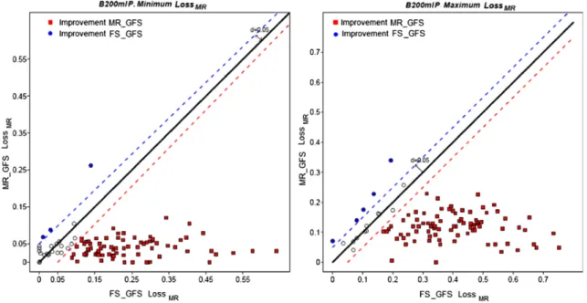
is uniform, we obtain the commonly used uniform precedence [55], which was originally defined for interval-valued data. This precedence is illustrated in Fig.1and in the examples that follow.

Example 1. LetA

= [

1

,

3

]

andB

= [

2

,

4

]

. If we assume thatP

(

a

,

b

)

is uniform in

[

1

,

3

] × [

2

,

4

]

(see Fig.1) we obtain P

(

{

(

a

,

b

)

:

a

≤

b

}

)

P

(

{

(

a

,

b

)

:

a

>

b

}

)

=

3

.

5

/

4

0

.

5

/

4

>

1 (53)

thusA

B.

Example 2. LetA

= [

1

,

5

]

andB

= [

1

.

9

,

4

]

. The application of the same principle produces P

(

{

(

a

,

b

)

:

a

≤

b

}

)

P

(

{

(

a

,

b

)

:

a

>

b

}

)

=

4

.

095 4

.

305

<

1 (54) thereforeB

A.

Depending on the shape of the membership functions ofAandBthe hypothesis about the uniform distribution of

(

a

,

b

)

still makes sense for fuzzy data. In this paper we have assumed that

(

a

,

b

)

→

Ul

(

A

),

r

(

A

)

×

l

(

B

),

r

(

B

)

,

(55)

wherel

(

A

)

,r

(

A

)

and the corresponding values forBare the bounds of the expectation of the fuzzy number, as defined in [21].

3.2.4. Fitness function

For crisp data, when thekth instance is presented to the classifier, the fitness of the winner rulewis penalized with a value that matches the risk of classifying this object,

fit

(

w

,

k

)

=

bqryk

.

(56)

It is remarked that the objective of this learning is to minimize the fitness (minimize the risk), contrary to the usual practice in this kind of algorithms, where the objective is maximizing the fitness (the number of well classified instances).

Before extending this expression to interval data, let us rewrite Eq. (56) as follows: fit

(

w

,

k

)

=

C

j=1

δj

,ykbqrj. (57)

For interval data, each ruleRrin the winner set is penalized with an interval-valued risk, because the true class of thekth

object can be perceived as a set of elements ofC. In this case, our knowledge about the fitness value is given by an extension of Eq. (57): fit

(

r

,

k

)

=

⎧ ⎨ ⎩ C j=1

γj

bqrj

|

γj

∈

δ

j,Ykand C j=1

γj

=

1 ⎫ ⎬ ⎭

,

(58)

where

δ

is a set-valued generalization of Dirichlet’s delta, that was defined in Eq. (18). Since the computation of the preceding expression is costly, we will enclose it in the set

fit

(

r

,

k

)

=

C

j=1

δj

,Ykbqrj. (59)

Let us clarify the meaning of this expression with a numerical example. Letqr=c2,Yk={c1,c3},C

= {

c1

,

c2

,

c3

}

, and let the matrixB=[bij] be B

=

0

[

0

.

8

,

1

] [

0

.

7

,

0

.

9

]

[

0

.

1

,

0

.

3

] [

0

.

1

,

0

.

15

] [

0

.

3

,

0

.

6

]

1

[

0

.

6

,

0

.

85

]

0

.

The fitness of therth ruke will be:

fit

(

r

,

k

)

= {{

0

,

1

}[

0

.

1

,

0

.

3

] + {

0

}[

0

.

1

,

0

.

15

] + {

0

,

1

}[

0

.

3

,

0

.

6

]} = {

0

.

1

,

0

.

3

,

0

.

6

}

.

For fuzzy data, each ruleRrin the support of the winner setWis penalized with the risk of their classification, which in turn

might be a fuzzy set, if the true class of thekth object is partially unknown: fit

(

r

,

k

)

=

C

j=1

δj

,Yk bqrj, (60)

where

δ

was defined in Eq. (29).

3.2.5. Generational scheme and genetic operators

This GFS operates by selecting two parents with the help of a double binary tournament, where the order between the fuzzy valued fitness function depends on the sign of the median of the difference of those random variables we have assumed

implicit in the fuzzy memberships, with hypothesis of independence and uniform distribution, as explained in the Section 3.2.3. These two parents are recombined and mutated with standard two-point crossover [45] and uniform mutation [44], respectively. After the application of crossover or mutation we search the individuals for the occurrence of chains where there exist ‘OR’ combinations involving all the linguistic terms of a variable. As we have mentioned, these chains are replaced by chains of zeroes, representing “do not care” terms.

The consequent with a lower risk is determined for each element of the offspring, according to the procedure in Section 3.2.1, and inserted into a secondary population, whose size is smaller than that of the primary population. The worse individuals of the primary population (again, according to the same precedence operator) are replaced by those in the secondary population at each generation.

Once these individuals have been replaced, the fitness assignment begins. Each rule keeps a fuzzy counter, which is zeroed first. The second step consists in determining the set of winner rules defined in Section3.1, for each instancekin the dataset. The counters of these winner rules are incremented the amount defined in Section3.2.4. After one pass through the training set, the values stored at these counters are the fitness values of the rules. Duplicate rules are assigned a high risk. The algorithm ends when the number of generations reaches a limit or there are not changes in the global risk in certain number of generations. A detailed pseudocode of the generational scheme has been included in Appendix5.

4. Numerical results

The experimental validation comprises nine datasets, originated in two problems related to linguistic classification sys-tems with imprecise data (diagnosis of dyslexia [49] and future performance of athletes [47]). We have asked the experts that helped us with these problems to express their preferences about the classification results either with intervals or linguistic values. We intend to show that the algorithm proposed in this paper is able to exploit the subjective costs given by the human experts and produce a fuzzy rule based classification system according to their preferences.

These datasets contain imprecision in both the input and the output variables. Regarding the imprecision in the output, those instances with uncertainties in the class label can be regarded as multi-label data [9]. Nevertheless, observe that we do not intend to predict the crisp or fuzzy sets of classes assigned to those instances; we interpret a multi-label instance as an individual whose category was not clear to the expert, but he/she knows for sure a set of classes that this instance does not belong to. For instance, when diagnosing dyslexia, there were cases where the psychologist could not decide whether a child had dyslexia or an attention disorder. This does not mean that we should label the child as having both problems; on the contrary, the most precise fact we can attest about this child is that he should not be classified as “not dyslexic”.

We have also observed that, in some cases, the use of a cost matrix produces rule bases that improve the results obtained with the same algorithm and a zero-one loss. We attribute this interesting result to the fact that the use of costs modifies the default exploratory behavior of the genetic algorithm, making that some regions of the input space with a low density of examples are able to source rules that are still competitive in the latter stages of the learning. This effect will be further studied later.

The structure of this section is as follows: in the first place, we will describe an experiment illustrating the differences between numerical, interval-valued and linguistic (fuzzy) costs from the point of view of the human expert. Second, the datasets are described, and the experimental setting introduced, including the cost matrices, the metrics used for evaluating the results and those mechanisms we have used for removing the uncertainty in the data (needed for comparing this algorithm to other classification systems that cannot use imprecise data). The compared results between the new GFS and other alternatives are included at the end of this part.

4.1. Illustrative example

We have carried a small experiment for assessing the coherence of a subjective assignment of costs in classification problems. Our experts were asked to provide either a numerical cost, or a range of numbers or a linguistic term for each type of misclassification, according to their own preferences.

Our catalog of linguistic terms comprises eleven labels, described in Table1, where their semantics are defined by means of trapezoidal fuzzy intervals, described in turn by four parameters (the lowest element of the support, the lowest element of the mode, the highest element of the mode, the highest element of the support). The left and rightmost terms “Absolutely low” and “Unacceptable” are crisp labels, following a requirement of one of the experts. Apart from this, experts were not explained this semantic; their choice was guided by the linguistic meaning they attributed to each label by themselves.

The experts we are working with, that is to say both the expert in athletism and the expert in dyslexia, found natural to use the linguistic terms. When they asked to use numbers or intervals they made a conversion table and used their prior linguistic selection to find an equivalent numerical score, to which they assigned an amplitude reflecting their uncertainty about the number. Generally speaking, there were large overlappings between their intervals. For example, an expert had not conflicts choosing the linguistic cost of misclassification “Fairly-high” between the eleven alternatives, but assigned to the same subjective cost the interval

[

0

.

55

,

0

.

85

]

. There was also consensus assigning the highest cost to those cases where the result of a misclassification had undesired consequences. Interestingly enough, if the experts are asked to use a scale

Table 1

Linguistic terms and parameters defining their membership functions. Linguistic term Fuzzy membership Absolutely-low (0,0,0,0) Insignificant (0,0.052,0.105,0.157) Very low (0.105,0.157,0.210,0.263) Low (0.210,0.263,0.315,0.368) Fairly-low (0.315,0.368,0.421,0.473) Medium (0.421,0.473,0.526,0.578) Medium-high (0.526,0.578,0.631,0.684) Fairly-high (0.631,0.684,0.736,0.789) High (0.736,0.789,0.842,0.894) Very-high (0.842,0.894,0.947,1) Unacceptable (1,1,1,1) Table 2

Answers of an expert when asked to assign a cost to certain misclassification.

Scale Interval Number Linguistic term

[0,1] [0.8,1] 1 High

[1,1000] [700,850] 800 High

different than

[

0

,

1

]

(between 1 and 1000, for instance) their judgement was different. As an example, in the Table2we have collected the responses of an expert that was asked, at different times, to assign a cost to certain misclassification:

In this example, the expert was consistent in the selection of a linguistic value, not so when selecting a numerical value: the first time he was asked, he chose the highest numerical cost (1) for a decision he did not associate the highest linguistic cost to. Furthermore, when the scale was changed, the numerical cost was different too, and in this last case this cost was similar to the corresponding trapezoidal fuzzy set in Table1. Generally speaking, we can conclude that the linguistic assignment of cost was preferred to the numerical assignment, and that a subjective assignment of numbers or ranges to costs produces less coherent results than linguistic values. This result will be illustrated later with numerical experiments: we will show that the classification systems obtained when the expert builds a linguistic cost matrix have a confusion matrix that is preferable to that of the rule base arising from the interval-valued cost matrix.

4.2. Description of the datasets

The datasets “Diagnosis of the Dyslexic” and “Athletics at the Oviedo University”, have been introduced in [49] and [47], respectively, and are available in the data set repository of keel-dataset (http://www.keel.es/datasets.php) [3,4]. Their description is reproduced here for the convenience of the reader.

Dyslexia can be defined as a learning disability in people with normal intellectual coefficient, and without further physical or psychological problems that can explain such disability. The dataset “Diagnosis of the Dyslexic” is based on the early diagnosis (ages between 6 and 8) of schoolchildren of Asturias (Spain), where this disorder is not rare. All schoolchildren at Asturias are routinely examined by a psychologist that can diagnose dyslexia (in Table3there is a list of the tests that are applied in Spanish schools for detecting this problem). It has been estimated that between 4% and 5% of these schoolchildren have dyslexia. The average number of children in a Spanish classroom is 25, therefore there are cases at most classrooms [2]. Notwithstanding the widespread presence of dyslexic children, detecting the problem at this stage is a complex process, that depends on many different indicators, mainly intended to detect whether reading, writing and calculus skills are being acquired at the proper rate. Moreover, there are disorders different than dyslexia that share some of their symptoms and therefore the tests not only have to detect abnormal values of the mentioned indicators; in addition, they must also separate those children which actually suffer dyslexia from those where the problem can be related to other causes (inattention, hyperactivity, etc.).

The problem “Athletics at the Oviedo University” comprises eight different datasets, whose descriptions are as follows: (1) Dataset “B200ml-I”: This dataset is used to predict whether an athlete will improve certain threshold in 200 meters.

All the indicators or inputs are fuzzy-valued and the outputs are sets.

(2) Dataset “B200mlP”: Same dataset as “B200mlI”, with an extra feature: the subjective grade that the trainer has assigned to each athlete. All the indicator are fuzzy-valued and the outputs are sets.

(3) Dataset “Long”: This dataset is used to predict whether an athlete will improve certain threshold in the long jump. All the features are interval-valued and the outputs are sets. The coach has introduced his personal knowledge. (4) Dataset “BLong”: Same dataset as “Long”, but now the measurements or inputs are defined by fuzzy-valued data,

obtained by reconciling different measurements taken by three different observers.

(5) Dataset “100ml”: Used for predicting whether a threshold in the 100 m sprint race is being achieved. Each measurement was repeated by three observers. The input variables are intervals and outputs are sets.

Table 3

Categories of the tests currently applied in Spanish schools for detecting dyslexia when an expert evaluates the children.

Category Test Description

Verbal comprehension BAPAE Vocabulary

BADIG Verbal orders

BOEHM Basic concepts

Logic reasoning RAVEN Color

BADIG Figures

ABC Actions and details

Memory Digit WISC-R Verbal-additive memory

BADIG Visual memory

ABC Auditive memory

Level of maturation ABC Combination of different tests Sensory-motor skills BENDER visual-motor coordination

BADIG Perception of shapes

BAPAE Spatial relations, shapes, orientation STAMBACK Auditive perception, rhythm HARRIS/HPL Laterality, pronunciation

ABC Pronunciation

GOODENOUGHT Spatial orientation, Body scheme

Attention Toulose Attention and fatigability

ABC Attention and fatigability

Reading–writing TALE Analysis of reading and writing

Table 4

Summary descriptions of the datasets used in this study.

Dataset Ex. Atts. Classes %Inst_classes

B200mlI 19 4 2 ([0.47,0.73],[0.26,0.52]) B200mlP 19 5 2 ([0.47,0.73],[0.26,0.52]) Long 25 4 2 ([36,64],[36,64]) BLong 25 4 2 ([36,64],[36,64]) 100mlI 52 4 2 ([0.44,0.63],[0.36,0.55]) 100mlP 52 4 2 ([0.44,0.63],[0.36,0.55]) B100mlI 52 4 2 ([0.44,0.63],[0.36,0.55]) B100mlP 52 4 2 ([0.44,0.63],[0.36,0.55]) Dyslexic-12 65 12 4 ([0.32,0.43],[0.07,0.16], [0.24,0.35],[0.12,0.35])

(6) Dataset “100mlP”: Same dataset as “100mlI”, but the measurements have been replaced by the subjective grade the trainer has assigned to each indicator (i.e.“reaction time is low” instead of “reaction time is 0.1 seg”).

(7) Dataset “B100mlI”: Same dataset as “100mlI”, but now the measurements are defined by fuzzy-valued data. (8) Dataset “B100mlP”: Same dataset as “100mlP”, but now the measurements are defined by fuzzy-valued data. A brief summary of the statistics of these problems is provided in Table4. The name, the number of examples (Ex.), number of attributes (Atts.), the classes (Classes) and the fraction of patterns of each class (%Inst_classes) of each dataset are displayed. Observe that these fractions are intervals, because the class labels of some instances are imprecise, and can be used for computing a range of imbalance ratios.

4.3. Experimental settings

All the experiments have been run with a population size of 100, probabilities of crossover and mutation of 0.9 and 0.1, respectively, and limited to 100 generations. The fuzzy partitions of the labels are uniform and their size is 5. All the imprecise experiments were repeated 100 times with bootstrapped resamples of the training set and where each partition of test contains 1000 tests.

For those experiments involving preprocessed data, the GFS proposed in [50] is used, with three nearest neighbors. This algorithm balances all the classes taking into account the imprecise outputs. This method of preprocessing is also applied to the 100 bootstrapped resamples of the training set.

Table 5

Interval cost matrices designed by a human expert in Athletics datasets.

True class Jump True class 100–200 m True class B100–B200 m

Estimated labels Estimated labels Estimated labels

0 1 0 1 0 1

0 0 [0.6,0.9] 0 0 0.8 0 0 [0.8,0.94]

1 0.5 0 1 0.4 0 1 [0.15,0.24] 0

Table 6

Linguistic cost matrices designed by a human expert in Athletics datasets.

True class Jump True class 100–200 m and B100–B200 m

Estimated labels Estimated labels

0 1 0 1

0 Absolutely-low Fairly-high 0 Absolutely-low High

1 Low Absolutely-low 1 Very low Absolutely-low

Table 7

Linguistic cost matrix designed by a human expert in Dyslexic’s dataset. True class Classifier

0 1 2 4

Dyslexic-12

0 Absolutely-low Medium Very-high Unacceptable

1 Fairly-low Absolutely-low Low Very-high

2 Unacceptable Medium Absolutely-low High

4 High High Low Absolutely-low

4.3.1. Matrix of misclassification costs

The cost matrices used in the different datasets of Athletics [47] are shown in Tables5and6. In both tables the expert preferred to discard a potentially good athlete (class 1) over accepting someone who is not scoring good marks (class 0). The actual costs depend on the event, as shown in Tables5(intervals) and6(linguistic terms). Observe that in Table5the costs are defined either by interval or crisp values; we commanded the experts to define the costs by means of numerical values, and to use intervals when they could not precise the numbers.

The Dyslexic’s dataset is more complex and the expert decided by herself that her numerical assignments were not reliable, recommending us a design based on her linguistic matrix instead. The initial design was intended to separate dyslexic children (“class 2”) from those in need of “control and review” (“class 1”) and those without the problem. This is akin to an imbalanced problem, albeit there were some problems derived from this initial assignment of costs. For instance, in the case that a child is not dyslexic (“class 0”) and the classifier indicates that he has a learning problem different than dyslexia (“class 4”), the misclassificacion cost was “Absolutely-low”, because the expert was understanding that the classifier would indicate that the child is not dyslexic. However, the expert did not take into account that, in this case, this child would be subjected to psychological treatment, which could potentially cause him certain disorders. The same situation happened when the child has an attention disorder and the classifier indicates that the child is dyslexic. In this case, the misclassification cost was “Very-high”, according to the idea that is was more important to mark off the dyslexic children than leaving a dyslexia case undetected. Again, the consequences can be negative for the misclassified child, thus a finer distinction is needed. The second design takes into account this possibilities, and is shown in the Table7.

4.3.2. Metrics for evaluating the results

The classification cost, when a zero-one loss is used, is the fraction of misclassified instances. For instance, regarding the confusion matrix of a two-classes problem,

Negative Prediction Positive Prediction

Negative class TN FP Positive class FN TP this cost is loss0−1

=

FP

+

FN TP

+

TN

+

FP

+

FN

.

(61)

Table 8

Misclassifications in the Athletics datasets from MR_GFS with a cost matrix defined by interval-valued and linguistic costs.

Dataset Interval-values Linguistic terms

C0asC1(FP) C1asC0(FN) C0asC1(FP) C1asC0(FN) 100mlI 1752 5363 1038 6228 100mlP 1609 4795 970 6078 B100mlI 975 6268 991 6258 B100mlP 1085 5590 1103 5558 Long 1785 3289 1638 3385 BLong 1891 3418 1609 3762 B200mlI 182 2511 182 2479 B200mlP 165 2570 164 2577 % 21.85 78.15 17.48 82.52

For evaluating this error with imprecise data we will use the same expressions introduced in Section2for the minimum risk problem (Eqs. (23) and (34)) with a cost matrixB

= [

1

−

δij

]

. Using this binary cost matrix we can also generalize the zero-one loss to multiclass problems either with crisp, interval or imprecise data.

For different cost matrices we will compare algorithms on the basis of the value lossMR

=

R, as defined in Eqs. (23) and

(34). Other commonly used metrics, like the Area Under the ROC Curve (AUC) [7,52] have not been used in this work because a suitable generalization to multi-class imprecise problems has not yet been proposed.

4.3.3. Heuristics for the removal of meta-information

For those comparisons involving statistical or intelligent classifiers unable to accept imprecise data, a procedure for removing the meta-information in the data is needed. The rules that will be used in this paper are as follows:

•

If the meta-information is in the input, each interval is replaced by its midpoint. In case the data is fuzzy, the midpoint of its modal interval is chosen instead.

•

If the imprecision is in the class label, each sample is replicated for the different alternatives. For instance, an example (x=2, c=A,B) is converted in two examples (x=2, c=A) and (x=2, c=B).

Observe that each time an example is replicated the remaining instances have to be repeated the number of times needed for preserving the statistical significance of each object. The drawback of this procedure is that problems which seem to be simple by the standards of crisp classification systems become complex datasets when the uncertainty is removed. For example, Dyslexic-12, with 65 instances and a high degree of imprecision, is transformed into a crisp dataset with thousands of instances.

4.4. Compared results

In this section we will compare the performance of the different alternatives in the design of the new GFS, and the results of this new GFS to those of different classifiers. The experiments are organized as follows:

(1) GFS with linguistic cost matrices vs. GFS with interval-valued costs. (2) GFS with zero-one loss vs. GFS with minimum risk-based loss. (3) A selection of crisp classifiers vs. GFS with minimum risk-based loss. (4) GFS for imbalanced data vs. GFS with risk-based loss.

4.4.1. Interval and fuzzy costs

With this experiment we compare the behaviors of the GFSs depending on numerical costs (interval-valued costs) to those depending on linguistic costs. We will study the confusion matrix of the classifiers obtained with interval-valued and fuzzy risks, using the matrices that the experts provided for each case. For computing a numerical confusion matrix we have applied the procedure described in Section4.3.3and extended the test set by duplicating the imprecise instances.

In the athletics problems, the coach prefers to label an athlete as not relevant (“class 0”) when he/she is relevant (“class 1”) than the opposite, thus the misclassification (“label aC1case as if it wasC0”) is preferred over (C0asC1). In Table8 we show that the percentage of misclassifications “C1asC0” achieved with the linguistic cost matrix is higher (82,52%) than that obtained with interval-valued costs (78,15%). Observe that we do not claim with this experiment that there is not a numerical or interval-valued set of costs that produces a classifier improving, in turn, this result: our point is that a linguistic description of weights models better the subjective preferences of the expert, and our system was able to exploit this linguistic description for evolving a rule base that follows the preferences of the user.

As mentioned in Section4.3.1, the expert in the field of dyslexia decided that her numerical assigments were not reliable. For comparing the results obtained after her selection of a numerical cost matrix (comprising intervals and real numbers)

Table 9

Misclassifications in the Dyslexic datasets from MR_GFS with a cost matrix defined by interval-valued and linguistic costs.

Dyslexic Interval-values Int.N. Linguistic terms Ling.N.

C0asC4 [0.6,0.9] 195 Unacceptable 124 C2asC0 1 62 Unacceptable 80 C4asC1 0.75 87 High 44 C2asC4 0.6 329 High 272 C1asC4 0.6 27 Very-high 16 C0asC2 0.7 5326 Very-high 5314 C2asC1 [0.3,0.35] 202 Medium 112 C0asC1 [0.2,0.4] 424 Medium 359 TotalN. – 6652 – 6321 Table 10

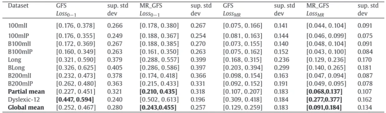
Behaviour of “GFS” and “MR_GFS” with respect to Loss0−1and LossMR.

Dataset GFS sup. std MR_GFS sup. std GFS sup. std MR_GFS sup. std

Loss0₋1 dev Loss0−1 dev LossMR dev LossMR dev

100mlI [0.176,0.378] 0.266 [0.178,0.380] 0.267 [0.075,0.166] 0.141 [0.044,0.104] 0.091 100mlP [0.176,0.355] 0.249 [0.188,0.367] 0.254 [0.081,0.163] 0.144 [0.046,0.099] 0.075 B100mlI [0.172,0.369] 0.267 [0.188,0.385] 0.270 [0.073,0.155] 0.140 [0.048,0.104] 0.091 B100mlP [0.160,0.349] 0.263 [0.161,0.350] 0.263 [0.075,0.162] 0.152 [0.043,0.100] 0.084 Long [0.321,0.590] 0.379 [0.288,0.557] 0.399 [0.168,0.315] 0.236 [0.129,0.236] 0.170 BLong [0.326,0.625] 0.405 [0.286,0.586] 0.397 [0.203,0.394] 0.299 [0.140,0.265] 0.181 B200mlI [0.232,0.473] 0.378 [0.174,0.418] 0.366 [0.098,0.154] 0.163 [0.047,0.094] 0.087 B200mlP [0.262,0.480] 0.363 [0.215,0.433] 0.331 [0.092,0.152] 0.191 [0.049,0.095] 0.078 Partial mean [0.227,0.451] 0.321 [0.210, 0.435] 0.318 [0.107,0.207] 0.183 [0.068,0.137] 0.107 Dyslexic-12 [0.447, 0.594] 0.240 [0.502,0.613] 0.196 [0.309,0.418] 0.184 [0.277,0.377] 0.162 Global mean [0.252,0.467] 0.280 [0.243,0.455] 0.257 [0.129,0.259] 0.183 [0.091,0.184] 0.134

Fig. 2. Behaviour of “GFS” and “MR_GFS” respect toLoss0−1in 100mlI.Left:Lower bounds.Right:Upper bounds.

with those obtained with the corresponding linguistic cost matrix we have built Table9. Each row “CpasCq” shows the

number of children for which the output of the classifier wasCpwhen the value should have beenCq. Observe that there are

improvements for all the combinations but “C2asC0”, and the global number of misclassifications is also reduced. 4.4.2. Comparison between GFSs using Loss0−1and LossMR

In this section the minimum error-based extended cooperative-competitive algorithm defined in [48] (labelled “GFS”) will be compared to the minimum risk-based GFS in this paper (labelled “MR_GFS”). Each rule base will be evaluated twice

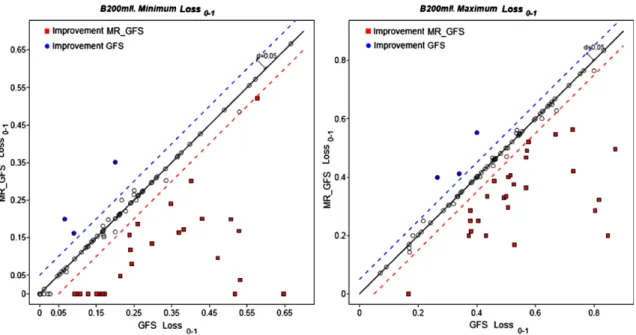
Fig. 3. Behaviour of “GFS” and “MR_GFS” respect toLoss0−1in B200mlI.Left:Lower bounds.Right:Upper bounds.

Fig. 4. Behaviour of the “GFS” and “MR_GFS” with respect toLossMRin 100mlI.Left:Lower bounds.Right:Upper bounds.

on the same test sets, using both a minimum-risk based criterion (LossMR) and a zero-one loss (Loss0−1). Observe that the zero-one loss is the fraction of misclassified examples, or in other words the minimum-error based criterion.

In the first place, let us compare the misclassification rate (Loss0−1) of “GFS” and “MR_GFS”. It was expected that the cost-based classifier obtained the worst results, since it has not been designed for optimizing the zero-one loss. Rather surprisingly, the first two columns of Table10(GFSLoss0−1and MR_GFSLoss0−1) contain evidence that the use of the new algorithm has improved the absolute number of misclassifications with respect to its minimum error-based counterpart in most datasets.

The statistical relevance of these differences has been graphically displayed in Figs.2and3. Each point in these figures represents one of the experiments. The abscissa is Loss0−1(i.e. the fraction of errors) of the first approach and the ordinate is same type of risk for the second procedure. That is to say, points over the diagonal (circles) are the cases where the minimum error-based classifier produced a better rule set. Since the risks are interval-valued in this example, the figures are divided