optimization for large-scale machine learning problems
Francois Fagan
Submitted in partial fulfillment of the requirements for the degree
of Doctor of Philosophy
in the Graduate School of Arts and Sciences
COLUMBIA UNIVERSITY
c
2018
Francois Fagan All Rights Reserved
Advances in Bayesian inference and stable
optimization for large-scale machine learning problems
Francois Fagan
A core task in machine learning, and the topic of this thesis, is developing faster and more accurate methods of posterior inference in probabilistic models. The thesis has two components. The first explores using deterministic methods to improve the efficiency of Markov Chain Monte Carlo (MCMC) algorithms. We propose new MCMC algorithms that can use deterministic methods as a “prior” to bias MCMC proposals to be in areas of high posterior density, leading to highly efficient sampling. In Chapter 2 we develop such methods for continuous distributions, and in Chapter 3 for binary distributions. The resulting methods consistently outperform existing state-of-the-art sampling techniques, sometimes by several orders of magnitude. Chapter 4 uses similar ideas as in Chapters 2 and 3, but in the context of modeling the performance of left-handed players in one-on-one interactive sports.
The second part of this thesis explores the use of stable stochastic gradient descent (SGD) methods for computing a maximum a posteriori (MAP) estimate in large-scale machine learning problems. In Chapter 5 we propose two such methods for softmax regression. The first is an implementation of Implicit SGD (ISGD), a stable but difficult to implement SGD method, and the second is a new SGD method specifically designed for optimizing a double-sum formulation of the softmax. Both methods comprehensively outperform the previous state-of-the-art on seven real world datasets. Inspired by the success of ISGD on the softmax, we investigate its application to neural networks in Chapter 6. In this chapter we present a novel layer-wise approximation of ISGD that has efficiently computable updates. Experiments show that the resulting method is more robust to high learning rates and generally outperforms standard backpropagation on a variety of tasks.
Table of Contents
List of Figures vii
List of Tables xi
1 Introduction 1
I Advances in Bayesian inference: Leveraging deterministic methods for
ef-ficient MCMC inference 5
2 Elliptical Slice Sampling with Expectation Propagation 6
2.1 Introduction . . . 6
2.2 Expectation propagation and elliptical slice sampling . . . 8
2.2.1 Elliptical slice sampling . . . 8
2.2.2 Expectation propagation . . . 10
2.2.3 Elliptical Slice Sampling with Expectation Propagation . . . 11
2.3 Recycled elliptical slice sampling . . . 13
2.4 Analytic elliptical slice sampling . . . 17
2.4.1 Analytic EPESS for TMG . . . 19
2.5 Experimental results . . . 20
2.5.1 Probit regression . . . 21
2.5.2 Truncated multivariate Gaussian . . . 22
2.5.3 Log-Gaussian Cox process . . . 24
2.6 Discussion and conclusion . . . 24
3.2 Annular augmentation sampling . . . 28
3.2.1 Annular Augmentations . . . 29
3.2.2 Generic Sampler . . . 31
3.2.3 Operator 2: Rao-Blackwellized Gibbs . . . 32
3.2.4 Choice And Effect Of The Prior ˆp . . . 34
3.3 Experimental results . . . 35
3.3.1 2D Ising Model . . . 36
3.3.2 Heart Disease Risk Factors . . . 39
3.4 Conclusion . . . 41
4 The Advantage of Lefties in One-On-One Sports 42 4.1 Introduction and Related Literature . . . 42
4.2 The Latent Skill and Handedness Model . . . 48
4.2.1 Medium-Tailed Priors for the Innate Skill Distribution . . . 49
4.2.2 LargeN Inference Using Only Aggregate Handedness Data . . . 51
4.2.3 Interpreting the Posterior ofL . . . 53
4.3 Including Match-Play and Handedness Data . . . 56
4.3.1 The Posterior Distribution . . . 57
4.3.2 Inference Via MCMC . . . 58
4.4 Using External Rankings and Handedness Data . . . 62
4.5 Numerical Results . . . 63
4.5.1 Posterior Distribution ofL . . . 64
4.5.2 On the Importance of Conditioning on Topn,N . . . 64
4.5.3 Posterior of Skills With and Without the Advantage of Left-handedness . . . 66
4.6 A Dynamic Model forL . . . 69
4.7 Conclusions and Further Research . . . 73
II Advances in numerical stability for large-scale machine learning problems 76
5 Stable and scalable softmax optimization with double-sum formulations 77
5.1 Introduction . . . 77
5.2 Convex double-sum formulation . . . 80
5.2.1 Instability of ESGD . . . 81
5.2.2 Choice of double-sum formulation . . . 82
5.3 Stable and scalable SGD methods . . . 83
5.3.1 Implicit SGD . . . 83 5.3.2 U-max method . . . 86 5.4 Experiments . . . 88 5.4.1 Experimental setup . . . 88 5.4.2 Results . . . 91 5.5 Conclusion . . . 94 5.6 Extensions . . . 94 6 Implicit backpropagation 95 6.1 Introduction . . . 95
6.2 ISGD and related methods . . . 97
6.2.1 ISGD method . . . 97
6.2.2 Related methods . . . 98
6.3 Implicit Backpropagation . . . 99
6.4 Implicit Backpropagation updates for various activation functions . . . 101
6.4.1 Generic updates . . . 101
6.4.2 Relu update . . . 102
6.4.3 Arctan update . . . 104
6.4.4 Piecewise-cubic function update . . . 104
6.4.5 Relative run time difference of IB vs EB measured in flops . . . 104
6.5 Experiments . . . 106
6.6 Conclusion . . . 109
IV Appendices 129
A Elliptical Slice Sampling with Expectation Propagation 130
A.1 Monte Carlo integration . . . 130
A.2 Markov Chain Monte Carlo (MCMC) . . . 130
A.3 Slice sampling . . . 131
B Annular Augmentation Sampling 132 B.1 Rao-Blackwellization . . . 132
B.2 2D-Ising model results . . . 132
B.2.1 LBP accuracy . . . 133
B.2.2 Benefit of Rao-Blackwellization . . . 133
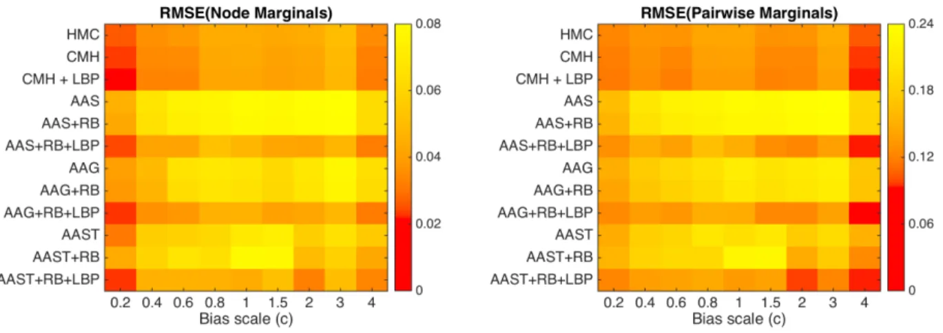
B.2.3 RMSE for node and pairwise marginals . . . 133
B.3 Heart disease dataset . . . 139
B.4 CMH + LBP sampler . . . 139
B.5 Simulated data . . . 141
B.5.1 d= 10 . . . 141
C The Advantage of Lefties in One-On-One Sports 143 C.1 Proof of Proposition 1 . . . 143
C.2 Rate of Convergence for Probability of Left-Handed Top Player Given Normal Innate Skills . . . 146
C.3 Difference in Skills at Given Quantiles with Laplace Distributed Innate Skills . . . . 150
C.4 Estimating the Kalman Filtering Smoothing Parameter . . . 151
D Stable and scalable softmax optimization with double-sum formulations 153 D.1 Comparison of double-sum formulations . . . 153
D.2 Proof of variable bounds and strong convexity . . . 155
D.3 Proof of convergence of U-max method . . . 158
D.4 Stochastic Composition Optimization . . . 160
D.5 Proof of general ISGD gradient bound . . . 161
D.6 Update equations for ISGD . . . 161
D.6.1 Single datapoint, single class . . . 162
D.6.2 Bound on step size . . . 167
D.6.3 Single datapoint, multiple classes. . . 168
D.6.4 Multiple datapoints, multiple classes . . . 171
D.7 Comparison of double-sum formulations . . . 175
D.8 Results over epochs . . . 177
D.9 L1 penalty . . . 179
D.10 Word2vec . . . 181
E Implicit Backpropagation 185 E.1 Derivation of generic update equations . . . 185
E.2 IB for convolutional neural networks . . . 187
E.3 Convergence theorem . . . 188
E.4 Experimental setup . . . 193
E.4.1 Datasets . . . 193
E.4.2 Loss metrics . . . 194
E.4.3 Architectures . . . 195
E.4.4 Hyperparameters and initialization details . . . 196
E.4.5 Learning rates . . . 196
E.4.6 Clipping . . . 197
E.5 Results . . . 197
E.5.1 Run times . . . 197
E.5.2 Results from MNIST and music experiments . . . 197
E.5.3 MNIST classification . . . 200
E.5.4 MNIST autoencoder . . . 203
E.5.5 JSB Chorales . . . 205
E.5.6 MuseData . . . 209
E.5.7 Nottingham . . . 211
E.5.8 Piano-midi.de . . . 213
List of Figures
1.1 Approaches to posterior inference in probabilistic models. The colored boxes and circles indicate the approaches used and developed in each chapter of the thesis. . . 2 2.1 ESS ellipse shown in dashed red. . . 10 2.2 The EP approximation is in teal and an EPESS elliptical slice is in dashed red. . . . 12 2.3 EPESS vs ESS: 400 samples of EPESS and ESS for a 2-d GaussianN(0, I) truncated
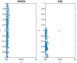
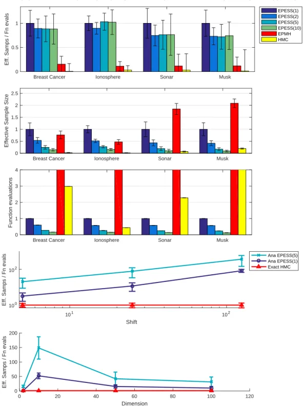
in a rectangular box {50≤x≤51,−1≤y≤1}. EPESS explores the parameter space effectively whereas ESS does not. . . 12 2.4 Plots of empirical results. In the top three plots all values are normalized so that
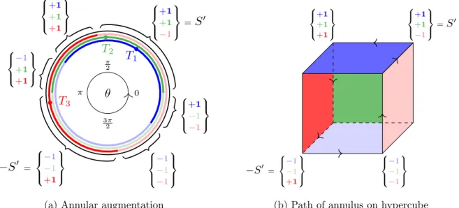
EPESS(1) has value 1. In the bottom 2 plots all values are normalized so that Exact-HMC has value 1. The naming convention: EPESS(J) denotes Recycled EPESS with J points sampled per slice. EPESS(1) denotes EPESS without recycling. Ana EPESS(J) denotes Analytic EPESS with J threshold levels per iteration. Error bars in plot 3 for all algorithms are effectively zero. . . 23 3.1 Diagram of the annular augmentation. (a) The auxiliary annulus. Each thresholdTi
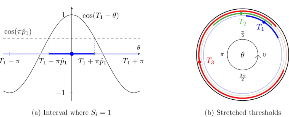
defines a semicircle where Si= +1, which is indicated by a darker shade. The value of S changes as θ moves around the annulus. (b) The implied path of the annulus on the binary hypercube. Hypercube faces are colored to match the annulus. . . 30 3.2 Augmentation with mean-field prior ˆp. (a) Equation (3.4) in graphical form; in blue,
the implied interval where s1 = 1 along the annulus. We denote ˆp1= ˆp(S1 = 1). (b) Stretched annular augmentation; cf. Figure 3.1a. . . 31
RB and AAG, AAG + RB increase their outperformance over all other samplers, including those using LBP (the LBP approximate degrades for W >0.6). . . 37 3.4 No bias is applied to any node making the target distribution bimodal, with the
modes becoming more peaked as strengthW is increased. All annular augmentation samplers very significantly outperform. . . 37 3.5 W is fixed to 0.2 and bias scale c is increased making the target distribution
uni-modal. HMC and CMH find the mode quickly, as do annular augmentation samplers that leverage LBP. That group outperforms annular augmentation samplers with no access to LBP. . . 38 3.6 Absolute error in estimating the log partition function ratio. Since there is zero bias,
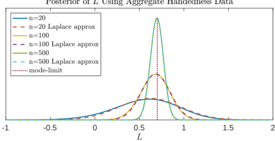
the LBP prior yields no additional benefit and so the results LBP driven samplers are omitted. . . 40 4.1 The value of limN→∞p(L | nl;n, N) as given by the r.h.s. of (4.9) for different
values of n. We assume an N(0,1) prior forp(L), a value of q = 11% and we fixed
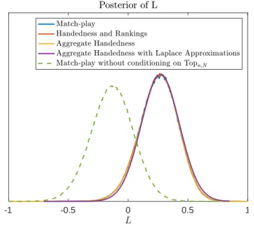
nl/n= 25%. The dashed vertical line corresponds toL∗ from (4.10) and the Laplace approximations are from (4.11). . . 53 4.2 Posteriors of the left-handed advantage, L, using the inference methods developed
in Sections 4.2, 4.3 and 4.4. “Match-play” refers to the results of MCMC inference using the full match-play data, “Handedness and Rankings” refers to MCMC infer-ence using only individual handedness data and external skill rankings, “Aggregate handedness” refers to (4.9) and “Aggregate handedness with Laplace Approxima-tion” refers to (4.9) but where the Laplace approximation in (4.11) substitutes for the likelihood term. “Match-play without conditioning on Topn,N” is discussed in Section 4.5.2. . . 65 4.3 Posterior distribution of Federer’s skill minus Nadal’s skill with and without the
advantage of left-handedness. . . 68 4.4 Marginal posterior distribution of Federer’s and Nadal’s skill, with and without the
advantage of left-handedness. . . 68
4.5 Posteriors of the left-handed advantage, Lt, computed using the Kalman filter / smoother. The dashed red horizontal lines (at 11% in the upper figure and 0 in the lower figure) correspond to the level at which there is no advantage to being left-handed. The error bars in the marginal posteriors ofLtin the lower figure correspond to 1 standard deviation errors. . . 72 5.1 Training log-loss vs CPU time. CPU time is marked by the number of epochs for
OVE, NCE, IS, ESGD and U-max (they all have virtually the same runtime). ISGD is run for the same CPU time as the other methods, but since it has a slightly different runtime per iteration, it will complete a different number of epochs. Thus when the x-axis is at 50, this indicates the end of the ISGD’s computation but not necessarily its 50th epoch. . . 92 5.2 Training log-loss on Eurlex for different learning rates. The x-axis denotes the
num-ber of epochs. . . 93 6.1 Illustration of the difference between ESGD and ISGD in optimizing f(θ) =θ2/2.
The learning rate is η= 1.75 in both cases. . . 98 6.2 Relu updates for EB and IB with µ = 0. The arrow tail is the initial value of θ>z
while the head is its value after the backpropagation update. Lower values are better.103 6.3 Training loss of EB and IB (lower is better). The plots display the mean performance
and one standard deviation errors. The MNIST-classification plot also shows an “exact” version of ISGD with an inner gradient descent optimizer. . . 107 6.4 Training loss of EB with clipping and IB with clipping on three dataset-architecture
pairs. . . 109 B.1 Estimated posterior distributions of Wij for 1 ≤ i < j ≤ 6 on the heart disease
dataset. The samples from each MH algorithm have had a normal distribution fit to them for easier comparison. “True” refers to the MH sampler where exact partition function ratio was used, whereas “CMH” and “AAS” refer to the approximate MH samplers for which the partition function ratio was approximated by CMH or AAS, respectively. . . 140
D.2 The x-axis is the number of epochs and the y-axis is the training set log-loss from (5.2).178
List of Tables
2.1 Datasets for probit experiments. . . 21 4.1 Proportion of left-handers in several interactive one-on-one sports [Flatt, 2008,
Loff-ing and Hagemann, 2016] with the relative changes in rank under the Laplace distri-bution for innate skills with q = 11%. Dropalone= n−nlnl·
1−q
q represents the drop in rank for a left-hander who alone gives up the advantage of being left-handed while Dropall = nqnl represents the drop in rank of a left-hander when all left-handers give up the advantage of being left-handed. . . 56 4.2 Probability of match-play results with and without the advantage of left-handedness.
The players are ordered according to their rank from the top ranked player (Djokovic) to the lowest ranked player (Lopez). A player’s rank is given by the posterior mean of his total skill,S. Each cell gives the probability of the lower ranked player beating the higher ranked player. Above the diagonal the advantage of left-handedness is included in the calculations whereas below the diagonal it is not. The left-handed players are identified in bold font together with the match-play probabilities that change when the left-handed advantage is excluded, i.e. when left- and right-handed players meet. . . 69
the MCMC samples generated using the full match-play data. The change in rank in the “Handedness and Rankings” column is computed using the MCMC samples given only individual handedness data and external skill rankings. The “Aggregate handedness” column uses the BTL ranking as the baseline and the change in rank is obtained by multiplying the baseline by the rank scaling factor of 1.36 from Table 4.1 and rounding to the closest integer. . . 70 5.1 Datasets with a summary of their properties. Where the number of classes, dimension
or number of examples has been altered, the original value is displayed in brackets. All of the datasets were downloaded fromhttp://manikvarma.org/downloads/XC/
XMLRepository.html, except WikiSmall which was obtained from http://lshtc.
iit.demokritos.gr/. . . 89 5.2 Tuned initial learning rates for each algorithm on each dataset. The learning rate in
100,±1,±2,±3/N with the lowest log-loss after 50 epochs using only 10% of the data
is displayed. ESGD applied to AmazonCat, Wiki10 and WikiSmall suffered from overflow with a learning rate of 10−3/N, but was stable with smaller learning rates
(the largest learning rate for which it was stable is displayed). . . 90 5.3 Relative log-loss of each algorithm at the end of training. The values for each dataset
are normalized by dividing by the corresponding Implicit log-loss. The algorithm with the lowest log-loss for each dataset is in bold. . . 92 6.1 IB relu updates . . . 103 B.1 LBP error for different values of W relating to Figure 3.3. The bias scale cis fixed
at 0.1. . . 134 B.2 LBP error for different values ofcrelating to Figure 3.5. Strength W is fixed at 0.2. 134 B.3 RMSE of node marginals estimate for increasing values ofW relating to Figure 3.4.
No bias is applied to any node. . . 135 B.4 Numerical values of RMSE (Node Marginals) for Figure 3.3. Bias scalec= 0.2 and
we increase the strength (W). . . 135
B.5 Numerical values of RMSE (Pairwise Marginals) for Figure 3.4. Bias scalec = 0.2 and we increase the strength (W). . . 136 B.6 Numerical values of RMSE (Node Marginals) for Figure 3.4. No bias is applied to
any node and we increase the strength (W). . . 136 B.7 Numerical values of RMSE (Pairwise Marginals) for Figure 3.4. No bias is applied
to any node and we increase the strength (W). . . 137 B.8 Numerical values of RMSE (Node Marginals) for Figure 3.5. We fix W = 0.2 and
the bias scalec is increased. . . 137 B.9 Numerical values of RMSE (Pairwise Marginals) for Figure 3.5. We fixW = 0.2 and
the bias scalec is increased. . . 138 D.1 Time in seconds taken to run 50 epochs. OVE/NCE/IS/ESGD/U-max with n =
1, m= 5 all have the same runtime. ISGD withn= 1, m= 1 is faster per iteration. The final column displays the ratio of OVE/.../U-max to ISGD for each dataset. . . 177 E.1 Data sources . . . 194 E.2 Data characteristics. An asterisk∗ indicates the average length of the musical piece.
88 is the number of potential notes in each chord. For information on the UCI classification datasets, see [Klambauer et al., 2017, Appendix 4.2]. . . 194 E.3 Theoretical and empirical relative run time of IB vs EB. Empirical measured on
AWS p2.xlarge with our basic Pytorch implementation. . . 198
Foremost, I would like to thank my supervisor Professor Garud Iyengar for guiding me through my PhD. Professor Iyengar has a seemingly boundless interest in all things. I always looked forward to our meetings and would often came away from them not only having gained greater academic understanding, but also with more knowledge (or questions!) about the world. I appreciate the freedom and support he has given me to explore my academic ideas, his generosity in offering fast and constructive feedback, and the patience he has shown me throughout the past five years.
One of the great pleasures of working in an interdisciplinary field like machine learning is the opportunity to learn from and collaborate with many people. Professors Krzysztof Choromanski, John Cunningham and Martin Haugh added an extra dimension to my work and were invaluable mentors through the PhD process. It was also a pleasure to learn and grow with Jalaj Bhandari and Hal Cooper, both fellow PhD candidates, through the projects we worked on together. I spent two of my summers at Bloomberg L.P. under Dr Kang Sun, Sergei Yurovski and Gary Kazantsev, who showed great faith in me and gave me my first exposure to industry. In particular, I’m deeply grateful for Gary Kazantsev arranging funding from Bloomberg for my PhD. My final summer was spent interning at Amazon.com where I was incredibly lucky to work with Dr Andres Ayala, Dr Michael Berry and Dr Evan Buntrock, who were all incredible mentors and good friends.
One of the most enjoyable aspects of my PhD were the excellent courses I took with my fel-low PhD candidates in my first few years at Columbia. Professors Cliff Stein, Donald Goldfarb, Ward Whitt, Garud Iyengar, Martin Haugh, Daniel Hsu, David Blei, Liam Paninski, Krzysztof Choromanski, John Cunningham and Shipra Agrawal exposed me to new ideas and provided me with a strong foundation for my research. It was also a rewarding experience to TA for and get to know Professors Soulaymane Kachani, Cyrus Mohebbi, Irene Song, Yuan Zhong, Soumyadip Ghosh, Martin Haugh and Ali Hirsa.
The staff in the Columbia IEOR department are always wonderful to work with. Thank you
to Darbi Leigh Roberts, Adina Berrios Brooks, Lizbeth Morales, Samuel Lee, Simon Mak, Yosimir Acosta, Gerald Cotiangco, Kristen Maynor, Shi Yee Lee, Jenny Mak, Jaya Mohanty and Carmen Ng for making my life easy. It was amazing to spend time and get to know many the other PhD candidates in the department. To keep the list short, I will just mention those who I have spent the most time with in our offices in room 321: Enrique Lelo de Larrea, Fengpei Li, Shuoguang Yang, Yuan Gao, Chaoxu Zhou, Camilo Hernandez and my desk-mate, Octavio Ruiz Lacedelli. I will miss your daily company.
I am also indebted to Professors John Cunningham, Adam Elmachtoub, Donald Goldfarb and Martin Haugh for agreeing to serve on my dissertation committee. They are all remarkable re-searchers for whom I have the greatest respect. I have been extremely fortunate to have had their presence in my academic life.
CHAPTER 1. INTRODUCTION 1
Chapter 1
Introduction
According to Box’s Loop [Box, 1976, Blei, 2014], the process of building probabilistic machine learning models involves looping through three tasks: model building, inferring hidden quantities and model criticism. The hope is that after cycling through these tasks a few times a good quality model will emerge that can then be used in practice.
This thesis focuses on improving the “inference” part of the loop. The goal here is to infer a posterior distribution, confidence interval or point estimate for the latent variables in a model, e.g. the parameters of a neural network.1 Ideally one would always calculate the full posterior
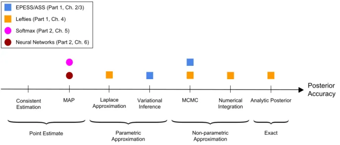
distribution of the latent variables. This gold standard is only achievable for some models where the posterior can be computed analytically, or for low-dimensional models where the posterior can be approximated using methods like Markov Chain Monte Carlo (MCMC). However, for more difficult problems, algorithms like MCMC can become impractically slow and other methods that are faster but return a less accurate posterior must be used instead. In Figure 1.1 we show a range of inference methods ordered by the accuracy of their posterior.
In this thesis we consider a diverse range of problems, each requiring new techniques that improve, combine or apply the approaches displayed in Figure 1.1. The thesis is divided into two parts, with the first part focused on developing efficient MCMC methods and the second part proposing new scalable algorithms for maximum a posteriori (MAP) estimation. The problems that we tackle will be fully introduced in their respective chapters. Here we give a short summary
Analytic Posterior MCMC Variational Inference Laplace Approximation MAP Posterior Accuracy Exact Non-parametric Approximation Parametric Approximation Point Estimate EPESS/ASS (Part 1, Ch. 2/3) Lefties (Part 1, Ch. 4) Softmax (Part 2, Ch. 5) Neural Networks (Part 2, Ch. 6)
Numerical Integration Consistent
Estimation
Figure 1.1: Approaches to posterior inference in probabilistic models. The colored boxes and circles indicate the approaches used and developed in each chapter of the thesis.
of each problem and make connections between the techniques that we use to solve them.
In the first part of this thesis we explore the use of deterministic methods to help model Bayesian systems and design efficient MCMC algorithms. Chapters 2 and 3 focus on performing posterior inference on common and important distributions like the truncated multivariate Gaussian, probit regression, Ising models and Boltzmann machines. MCMC techniques remain the gold standard for approximate Bayesian posterior inference as they are guaranteed to converge to the true posterior. However, their onerous runtime and sensitivity to tuning parameters often force one to use faster, but less accurate, deterministic approximations. Our high-level insight is that these deterministic methods can extract information about the posterior that can be used to construct highly efficient MCMC algorithms.
The challenge here is to: (i) design MCMC methods that can effectively harness information from deterministic methods, and (ii) identify deterministic methods that yield the most useful information. We address(i) by developing MCMC methods that can use the deterministic approx-imate posterior as a “prior” to bias their proposals to be in areas of high posterior density. The appropriate choice of deterministic method in(ii) is key to making the prior strong and likelihood weak, putting the MCMC algorithms in the regime where they are most efficient.
CHAPTER 1. INTRODUCTION 3
In Chapter 2 we develop this approach for continuous distributions, combining the deterministic approximation offered by expectation propagation with elliptical slice sampling, a state-of-the-art MCMC method. Chapter 3 extends the methodology to binary distributions. In order to harness the posterior yielded by belief propagation we invent an auxiliary variable MCMC scheme that samples from an annular augmented space, translating to a great circle path around the hyper-cube of the binary sample space. For both the continuous and binary cases the resulting MCMC algorithms consistently outperform the previous state-of-the-art MCMC methods, sometimes by multiple orders of magnitude.
Chapter 4 uses similar ideas, but in the context of modeling the performance of lefties in one-on-one interactive sports. Unlike the other chapters in this thesis that focus solely on inference, Chapter 4 involves all three tasks in Box’s Loop: model building, inferring hidden quantities and model criticism. The major challenge in this problem is that match-play data is only available for top ranked players, a fact that we explicitly build into our Bayesian model. Our key insight is that a deterministic approximation of the latent advantage of left-handedness (our main variable of interest) can be derived which only depends on the tail-length of the skill distribution. This deterministic approximation can then be used to inform the design of the Bayesian model, define a proposal distribution for a Metropolis-Hastings sampler and enable efficient inference of the advantage of left-handedness over time using a Kalman filter. The result is the first set of Bayesian inference techniques for inferring the advantage of left-handedness in one-on-one interactive sports where only data on top players is available.
The second part of this thesis explores the use of stable SGD methods for computing the max-imum a posteriori probability (MAP) of large-scale machine learning problems. The two problems we focus on are softmax optimization and neural network training. Both softmax and neural net-work models rely on having large amounts of data to make accurate predictions. This large amount of data results in there being a large number of terms in the MAP objective. Stochastic Gradient Descent (SGD) is the method of choice for such problems, as its run time per iteration is inde-pendent of the number of terms in the objective. However, the downside of SGD is that it can be unstable and require extensive tuning of the learning rate to ensure good performance.
Implicit SGD (ISGD) is an SGD method that is both stable and robust to the learning rate. The problem is that ISGD is typically difficult to implement as its update equation is highly
non-trivial. In this work we show that it is possible to apply ISGD to the softmax and neural networks. In Chapter 5 we show that the ISGD updates for a double-sum representation of the softmax can be reduced to a univariate problem that can be solved using a bisection method. We also propose another stable SGD method specifically designed for the softmax, which we call U-max. In Chapter 6 we explore the application of ISGD to neural network training. The ISGD updates are too expensive to compute exactly for neural networks. However, with carefully constructed approximations, the updates can be simplified and solved efficiently. Our proposed methods for softmax and neural network optimization are more stable, more robust and empirically converge faster than other SGD methods. The result is a more reliable set of methods for solving these large-scale problems.
In summary, this thesis has two parts. The first part explores the use of deterministic “priors” to speed up MCMC and the second develops new implementations of ISGD to improve the stability of MAP estimation in large-scale problems. The result is a new set of methods which improve the accuracy, speed and reliability of machine learning inference across a range of important and widely used models including: the truncated multivariate Gaussian, probit regression, Ising models, Boltzmann machines, softmax models and neural networks.
Notation
The first part of the thesis focuses on inference in explicitly Bayesian probabilistic models. Here random variables will be denoted by capital letters (e.g. X) and their values by lowercase letters (e.g. x). The exception is Greek letters (e.g. ν) where the lower case is used for both the random variables and values. Whether a Greek letter denotes a random variable or value will either be clear from the context or will be specified in the text.
For the second part of the thesis, where we are interested in MLE, lowercase letters will denote scalars or vectors while uppercase letters will refer to matrices.
5
Part I
Advances in Bayesian inference:
Leveraging deterministic methods for
Chapter 2
Elliptical Slice Sampling with
Expectation Propagation
2.1
Introduction
Exact posterior inference in Bayesian models is rarely tractable, a fact which has prompted vast amounts of research into efficient approximate inference techniques. Deterministic methods such as the Laplace approximation, Variational Bayes, and Expectation Propagation offer fast and analyti-cal posterior approximations, but introduce potentially significant bias due to their restricted form which cannot capture important characteristics of the true posterior. Markov Chain Monte Carlo (MCMC) methods represent the target posterior with samples, which while asymptotically exact, can be slow, require substantial tuning, and perform poorly when variables are highly correlated.
Conceptually, these two techniques can be combined to great benefit: if a deterministic approx-imation can cover the true posterior mass accurately, then a subsequent MCMC sampler should be much faster and be less susceptible to inefficiency due to correlation (if the deterministic approxi-mation has captured this correlation). In practice, however, this is quite difficult. First, both the Laplace and Variational Bayesian approximations yield a local approximation of the posterior (in Variational Bayes this is sometimes called theexclusiveproperty of optimizing the Kullback-Liebler divergence from the approximation to the true posterior [Minka, 2005]). While excellent in many situations, this property is inappropriate for initializing an MCMC sampler, since it will be very difficult for that sampler to explore other areas of posterior mass (e.g., other modes). Expectation
CHAPTER 2. ELLIPTICAL SLICE SAMPLING WITH EXPECTATION PROPAGATION 7
Propagation (EP, [Minka, 2001]), on the other hand, is typically derived as an inclusive approxi-mation that, at least approximately, attempts to match the global sufficient statistics of the true posterior (most often the first and second moments, producing a Gaussian approximation). Such a choice is a superior basis for an MCMC sampler.
Secondly, we require a sensible choice of MCMC sampler so as to leverage a deterministic approximation like EP. Given an unnormalized target distributionp∗(X), we can write
p∗(X) = pˆ(X)p ∗(X) ˆ
p(X) ≡ pˆ(X) ˆL(X)
for any ˆp, which allows us to treat the true posteriorp∗ as the product of an effective prior ˆp and likelihood ˆL=p∗/pˆ. We then have freedom to choose ˆp, which we will set to be the deterministic (Gaussian) posterior approximation from EP. Amongst all MCMC methods, Elliptical Slice Sam-pling (ESS, [Murray et al., 2010]) handles the above reformulations seamlessly. ESS has become an important and generic method for posterior inference with models that have a strong Gaussian prior. It inherits the attractive properties of slice sampling generally [Neal, 2003], and notably lacks tuning parameters that are often highly burdensome in other state-of-the-art methods like Hamiltonian Monte Carlo (HMC; Neal et al. [2011]). The critical observation is that if EP provides a quality posterior approximation ˆp ≈p∗, the likelihood term ˆL will be weak, which puts ESS in the regime where it is most efficient. What results is a new MCMC sampler that combines EP and ESS, is faster than state-of-the-art samplers like HMC, and is able to explore the parameter space efficiently even in the presence of strong dependency among variables.
The outline of the chapter is as follows. In Section 2.2, we propose Expectation Propagation based Elliptical Slice Sampling (EPESS) where we justify the use of EP as the “prior” for ESS. In Section 2.3, we investigate a method to improve the overall run time of ESS by sampling multiple points each iteration. It reduces the average number of shrinkage steps giving it a computational advantage. We call it Recycled ESS and integrate it with EPESS to further increase its efficiency. We extend our method toAnalytic Elliptical Slice Samplingin Section 2.4. As the name suggests, we can analytically find the region corresponding to a slice and sample uniformly from it. In addition to decorrelating samples, it offers the computational advantage of avoiding expensive shrinkage steps. It is applicable to only a few target distributions and we illustrate it, in the context of EPESS, for the linear Truncated Multivariate Gaussian (TMG). We offer an empirical evaluation
of EPESS (Section 2.5), which shows an order of magnitude improvement over the state-of-the art MCMC methods for TMG and probit models.
2.2
Expectation propagation and elliptical slice sampling
In this section we introduce our combined EP and ESS sampling method. We begin with background of the two building blocks of this method, to place them in context of current literature. Further background on Monte Carlo, MCMC and slice sampling methods is provided in Appendix A.
2.2.1 Elliptical slice sampling
There are many problems where dependency between latent variables is induced through a Gaussian prior, for example in Gaussian Processes. Elliptical Slice Sampling (ESS, [Murray et al., 2010]) is specifically designed for efficiently sampling from such distributions and is considered state-of-the-art on these problems. ESS considers posteriors of the form
p∗(X) ∝ N(X; 0,Σ)· L(X) (2.1) whereL is a likelihood function and N(0,Σ) is a multivariate Gaussian.
ESS is a variant of slice sampling [Neal, 2003] that takes advantage of the Gaussian prior to improve mixing time and eliminate parameter tuning. At the beginning of each iteration of ESS two random variables are sampled. The first is the slice heightY =ywhich is uniformly distributed over [0,L(x)], whereX=xis the current sample. The second variableν is sampled from the prior
N(0,Σ) and, together with the current samplex, defines an ellipse:
x0(θ) =xcos(θ) +νsin(θ). (2.2) The next point in the Markov chain will be sampled from this ESS ellipse. To do so, a one-dimensional angle bracket [θmin, θmax] of length 2π is proposed containing the point θ= 0
(corre-sponding to the current point x). The bracket is then shrunk toward θ= 0 until a point is found within the bracket that satisfies L(x0(θ)) ≥ y. This point is accepted as the next point in the Markov chain. The pseudocode for ESS is given in Algorithm 1.
ESS is known to work well when the prior aligns with the posterior and the likelihood is weak [Murray et al., 2010, Section 2.5]. The most extreme case is when the likelihood is a constant and
CHAPTER 2. ELLIPTICAL SLICE SAMPLING WITH EXPECTATION PROPAGATION 9
Algorithm 1:Elliptical Slice Sampling
Input : Log-likelihood function (logL), initial point x(0) ∈Rd, priorN(0,Σ), number of iterations N
Output: Samples from Markov Chain (x(1), x(2), ..., x(N))
1 for i= 1 to N do
2 Choose ellipse: ν ∼ N(0,Σ) 3 Log-likelihood threshold:
u∼Uniform[0,1]
logy←logL(x(i−1)) + logu
4 Define initial bracket:
θmax ∼Uniform[0,2π]
θmin ←θ−2π
5 do
6 Draw proposal:
θ∼Uniform [θmin, θmax]
x0 ←xcos(θ) +νsin(θ) 7 Shrink bracket:
8 if θ <0then θmin ←θ 9 elseθmax←θ
10 whilelogL(x0)<logy 11 Accept point: x(i)←x0 12 end
13 return (x(1), x(2), ..., x(N))
p∗(X) ∝ N(X; 0,Σ). In this case the first point proposed on the ESS ellipse is always accepted, and the Markov chain mixes fast. However, when this is not the case then ESS can perform poorly, as we demonstrate below.
Figure 2.1 illustrates the problem when the prior and the posterior do not align: here we have a N(0, I) prior with a Bernoulli likelihood L(x) =1(x ∈A) for some rectangle A. The posterior is a truncated Gaussian within A. In this example we have placed A away from the origin, with
CHAPTER 2. ELLIPTICAL SLICE SAMPLING WITH EXPECTATION PROPAGATION 10
the result that most of the posterior density lies vertically on the left boundary of the rectangle. Accordingly, a good sampler should be able to make large vertical moves to effectively explore the posterior mass.
servation is that, if EP provides a quality posterior
ap-proximation
p
ˆ
⇡
p
⇤, the likelihood term
L
ˆ
will typically
be weak, which puts ESS in the regime where it is most
efficient.
What results is a new MCMC sampler that combines
EP and ESS, is faster than state-of-the-art samplers like
HMC, and is able to explore the parameter space
effi-ciently even in the presence of strong dependency among
variables. Specifically, our contributions include:
1. In Section 2, we propose
Expectation Propagation
based Elliptical Slice Sampling (EPESS)
where we
justify the use of EP as the “prior” for ESS.
2. In Section 3, we investigate a method to improve
the overall run time of ESS by sampling multiple
points each iteration. It reduces the average number
of shrinkage steps giving it a computational
advan-tage. We call it
Recycled ESS
and integrate it with
EPESS to further increase its efficiency.
3. We extend our method to
Analytic Elliptical Slice
Sampling
in Section 4. As the name suggests, we
can analytically find the region corresponding to
a slice and sample uniformly from it. In
addi-tion to decorrelating samples, it offers the
compu-tational advantage of avoiding expensive shrinkage
steps. It is applicable to only a few target
distribu-tions and we illustrate it, in the context of EPESS,
for linear Truncated Multivariate Gaussian (TMG)
quadrature.
4. We offer empirical evaluation of EPESS
(Sec-tion 5), which show an order of magnitude
improve-ment over the state-of-the art MCMC methods for
TMG and probit models.
2 EXPECTATION PROPAGATION AND
ELLIPTICAL SLICE SAMPLING
In this section we introduce our combined EP and ESS
sampling method. We begin with background of the two
building blocks of this method, to place them in context
of current literature.
2.1 ELLIPTICAL SLICE SAMPLING
There are many problems where dependency between
la-tent variables is induced through a Gaussian prior, for
ex-ample in Gaussian Processes. Elliptical Slice Sampling
(ESS, [Murray et al., 2010]) is specifically designed for
ers posteriors of the form
p
⇤(
x
) =
1
Z
N
(
x
;
0
,
⌃
)
L
(
x
)
(1)
where
L
is a likelihood function,
N
(
0
,
⌃
)
is a
multivari-ate Gaussian prior and
Z
is the normalizing constant.
ESS is a variant of slice sampling [Neal, 2003] that takes
advantage of the Gaussian prior to improve mixing time
and eliminate parameter tuning. At the beginning of each
iteration of ESS two random variables are sampled. The
first is the slice height
y
which is uniformly distributed
over
[0
,
L
(
x
)]
, where
x
is the current sample. The second
variable
⌫
is sampled from the prior
N
(
x
;
0
,
⌃
)
and,
to-gether with the current sample
x
, defines an ellipse:
x
0(
✓
) =
x
cos(
✓
) +
⌫
sin(
✓
)
.
(2)
Next, a one-dimensional angle bracket
[
✓
min, ✓
max]
of
length
2
⇡
is proposed containing the point
✓
= 0
(cor-responding to the current point
x
). The bracket is then
shrunk toward
✓
= 0
until a point is found within the
bracket that satisfies
L
(
x
0(
✓
))
> y
. This point is
ac-cepted as the next point in the Markov chain.
ESS is known to work well when the prior aligns with
the posterior and the likelihood is weak [Murray et al.,
2010, Section 2.5]. However, when this is not the case
then ESS can perform poorly, as we demonstrate below.
Figure 1 illustrates the problem when the prior and the
posterior do not align: here we have a
N
(
0
,
I
)
prior with
an observed Bernoulli likelihood
L
(
x
) =
1
(
x
2
A
)
for
some rectangle
A
. The posterior is a truncated
Gaus-sian within
A
. In this example we have placed
A
away
from the origin, with the result that that most of the
pos-terior density lies vertically on the left boundary of the
box. Accordingly, a good sampler should be able to make
large vertical moves to effectively explore the posterior
mass.
⌫
x
A
Figure 1: ESS ellipse shown in dashed red.
As the likelihood rectangle
A
moves further right, the
posterior moves away from the prior. As a result most
of the points proposed on the ellipse will not lie in
A
, so
more shrinkage steps will be necessary until a point is
accepted, leading to an inefficient algorithm. Moving
A
Figure 2.1: ESS ellipse shown in dashed red.
As the likelihood rectangle Amoves further right, the posterior moves away from the prior. As a result, most of the points proposed on an ESS ellipse will not lie in A, so more shrinkage steps will be necessary until a point is accepted, making ESS inefficient. MovingA further to the right also makes the ESS ellipse more eccentric which prevents vertical movement, resulting in further inefficiency.
The other pathology afflicting ESS is that of strong likelihoods. This happens when L(x) is extremely large in regions of non-negligible posterior density. Once the sampler is in such a region, only with low probability will it be able to accept points proposed outside the region, hence it will get stuck. This will occur, for instance, when the prior underestimates the variance of the posterior andL(x) becomes large in the tails. We refer the reader to an extended explanation of this effect in [Nishihara et al., 2014, Sec. 3]. Indeed, this motivates our choice of EP as a prior, since Variational Bayes and Laplace approximations are known to often underestimate posterior variance whereas EP does not [Minka, 2005]. This is the same reason why using EP as a proposal distribution in an importance sampler yields a lower variance estimate than if Variational Bayes is used [Minka, 2005, App. E].
We address both these problems by choosing an EP prior for ESS. How to incorporate EP into ESS is explained in Section 2.2.3.
2.2.2 Expectation propagation
Expectation Propagation (EP) is a method for computing a Gaussian approximation q to a given distributionp∗ by iteratively matching local moments and then updating the global approximation
CHAPTER 2. ELLIPTICAL SLICE SAMPLING WITH EXPECTATION PROPAGATION 11
via a so-called ‘tilted’ distribution [Minka, 2001]. At termination the distribution q minimizes a global objective that approximates the Kullback-Liebler divergenceKL(p∗||q) [Wainwright and Jor-dan, 2008]. The resulting Gaussian approximation is aninclusive estimate ofp∗that approximately matches its zeroth, first, and second moments.
Although EP has few theoretical guarantees [Dehaene and Barthelm´e, 2015], it is known to be relatively accurate for many models including the truncated multivariate gaussian [Cunning-ham et al., 2011], probit and logistic regression [Nickisch and Rasmussen, 2008], log-Gaussian Cox processes [Ko and Seeger, 2015], and more [Minka, 2001]. It is also known to have superior perfor-mance compared to the Laplace approximation and Variational Bayes in terms of approximating marginal distributions accurately [Kuss and Rasmussen, 2005, Cseke and Heskes, 2011, Deisenroth and Mohamed, 2012].
2.2.3 Elliptical Slice Sampling with Expectation Propagation
As outlined in Section 2.1, we can incorporate a posterior approximation ˆpas a proposal distribution for ESS. We do so by defining:
p∗(X) = pˆ(X)p ∗(X) ˆ
p(X) = pˆ(X) ˆL(X) (2.3) wherep∗ is the posterior distribution of interest from (2.1), ˆp is our new prior and ˆL=p∗/pˆis our new likelihood.
As explained in Section 2.2.1, for ESS to work well, ˆp should have two desirable properties:
(i) It should approximate the posterior p∗. The most obvious candidates for ˆp includes Laplace, Variational Bayes and EP approximations,(ii) It should ensure that the new likelihood ˆL =p∗/pˆ is weak, in the sense as described in Section 2.2.1. Using either Laplace or Variational Bayes may result in large values of ˆL in the tails due to variance underestimation, which could cause the sampler to get stuck. The more inclusive nature of the EP estimate, on the other hand, makes it a sensible choice to obtain a Gaussian posterior approximation ˆp.
The formulation in (2.3) is intimately related to importance sampling where p∗ would be the target distribution and ˆp the proposal distribution. The properties that make EP a good prior for ESS also make EP a good proposal distribution for importance sampling [Minka, 2005, App. E]. Indeed, the EPESS algorithm may be thought of as an MCMC version of importance sampling.
CHAPTER 2. ELLIPTICAL SLICE SAMPLING WITH EXPECTATION PROPAGATION 12
To demonstrate the power of EPESS we return to the problematic example given in Figure 2.1. Using the EP approximation we can shift our “prior” ˆp to align with the posterior density p∗ on the left side of the likelihood rectangle A. The ESS ellipses become short and vertical, allowing ESS to mix efficiently. This is illustrated in Figure 2.2. To demonstrate the difference in the sampling behavior between EPESS and ESS, Figure 2.3 plots 400 samples from both EPESS and ESS. EPESS is clearly superior as it manages to explore the entire distribution whereas ESS does not.
inefficiency.
The other pathology afflicting ESS is that of strong
likeli-hoods. This happens when
L
(
x
)
is extremely large in
re-gions of non-negligible posterior density. Once the
sam-pler is in such a region, only with low probability will
it be able to accept points proposed outside the region,
hence it will get stuck. This will occur, for instance,
when the prior underestimates the variance of the
pos-terior and
L
(
x
)
becomes large in the tails. We refer the
reader to an extended explanation of this effect in
[Nishi-hara et al., 2014]. Indeed, this motivates our choice of
EP as a prior, since Variational Bayes and Laplace
ap-proximations are known to often underestimate posterior
variance whereas EP does not [Minka, 2005].
We address both these problems by choosing an EP prior
(Section 2.2) for ESS. How to incorporate EP into ESS
is explained in Section 2.3.
2.2 EXPECTATION PROPAGATION
Expectation Propagation (EP) is a method for finding a
Gaussian approximation
q
to a given distribution
p
⇤by
it-eratively matching local moments and then updating the
global approximation via a so-called ‘tilted’ distribution
[Minka, 2001]. At termination the distribution
q
will
op-timize a global objective that approximates the
Kullback-Liebler divergence
KL
(
p
⇤||
q
)
[Wainwright and Jordan,
2008]. The resulting Gaussian approximation is an
inclu-sive
estimate of
p
⇤that approximately matches its zeroth,
first, and second moments.
Although EP has few theoretical guarantees [Dehaene
and Barthelm´e, 2015], it is known to be accurate for
many models including truncated multivariate gaussian
[Cunningham et al., 2011], probit and logistic regression
[Nickisch and Rasmussen, 2008], log-Gaussian Cox
pro-cesses [Ko and Seeger, 2015], and more [Minka, 2001].
It is also known to have superior performance compared
to the Laplace approximation and Variational Bayes in
terms of approximating marginal distributions accurately
[Kuss and Rasmussen, 2005, Cseke and Heskes, 2011,
Deisenroth and Mohamed, 2012].
2.3 ELLIPTICAL SLICE SAMPLING WITH
EXPECTATION PROPAGATION
As outlined in Section 1, we incorporate a posterior
ap-proximation
p
ˆ
as a proposal distribution for ESS. We do
so by defining:
p
⇤(
x
) = ˆ
p
(
x
)
p
⇤
(
x
)
ˆ
p
(
x
)
= ˆ
p
(
x
) ˆ
L
(
x
)
(3)
lihood. As explained in Section 2.1, for ESS to work
well,
p
ˆ
should have two desirable properties:
(i)
It should
approximate the posterior
p
⇤. The most obvious
candi-dates for
p
ˆ
includes Laplace, Variational Bayes and EP
approximations,
(ii)
It should ensure that the new
like-lihood
L
ˆ
=
p
⇤/
p
ˆ
is weak, in the sense as described in
Section 2.1. Using either Laplace or Variational Bayes
may result in large values of
L
ˆ
in the tails due to
vari-ance underestimation, which could cause the sampler to
get stuck. The more inclusive nature of the EP estimate,
on the other hand, makes it a sensible choice to obtain a
Gaussian posterior approximation
p
ˆ
.
To demonstrate the power of this approach we return to
the problematic example given in Figure 1. Using the EP
approximation we can shift our prior to align with the
posterior density on the left side of the likelihood
rect-ange
A
. The ellipses become short and vertical, allowing
ESS to mix efficiently. This is illustrated in Figure 2.
To demonstrate the difference in the sampling behavior
between EPESS and ESS, Figure 2.3 plots 400 samples
from both EPESS and ESS. EPESS is clearly superior
and manages to explore the entire distribution whereas
ESS moves consistently less.
x
⌫
Figure 2: The EP approximation is in teal and an EPESS
elliptical slice is in dashed red.
The idea of Equation (3) is not unique to this paper.
Nishihara et al. [2014] use a similar construction where
the Gaussian approximation is learned from samples.
Al-though this has the advantage of not relying on EP to do
moment matching, it requires parallelism and expensive
moment calculations. EPESS will be simpler and more
efficient when an accurate EP approximation is available.
Braun and Bonfrer [2011] also have a similar method
where they use the Laplace approximation, which as
dis-cussed, is a poor choice. We remark that using Power EP
approximations is also a viable choice for a prior, a point
that we will return to in Section 6.
Figure 2.2: The EP approximation is in teal and an EPESS elliptical slice is in dashed red.
x 50 50.5 51 y -1 -0.8 -0.6 -0.4 -0.2 0 0.2 0.4 0.6 0.8 1 EPESS x 50 50.5 51 y -1 -0.8 -0.6 -0.4 -0.2 0 0.2 0.4 0.6 0.8 1 ESS
Figure 2.3: EPESS vs ESS: 400 samples of EPESS and ESS for a 2-d Gaussian N(0, I) truncated in a rectangular box {50≤x≤51,−1≤y≤1}. EPESS explores the parameter space effectively whereas ESS does not.
The idea of (2.3) is not unique to this paper. Nishihara et al. [2014] use a similar construc-tion where the Gaussian approximaconstruc-tion is learned from samples. Although their method has the
CHAPTER 2. ELLIPTICAL SLICE SAMPLING WITH EXPECTATION PROPAGATION 13
advantage of not relying on EP to do moment matching, it requires parallelism and expensive moment calculations. EPESS will be simpler and more efficient when an accurate EP approx-imation is available. Braun and Bonfrer [2011] also have a similar method where they use the Laplace approximation, which as discussed above, is a poor choice. We remark that using Power EP approximations is also a viable choice for a prior, a point that we will return to in Section 2.6.
2.3
Recycled elliptical slice sampling
In this section we show how to sampleJ >1 points each ESS iteration without a significant increase in computational complexity. This idea is inspired by the work of Nishimura and Dunson [2015] on HMC. In that work an HMC algorithm is devised which “recycles” the intermediate points as valid samples from the target distribution. We borrow the phrase “recycling” from them and call our method Recycled Elliptical Slice Sampling.
Recall from Section 2.2.1 that in every ESS iteration, we propose points along an ellipse within an angle bracket, which is iteratively shrunk, until a point is accepted. In Recycled ESS, we don’t stop after accepting the first point but continue to propose points starting from the last angle bracket used. This procedure is continued until J points are accepted. One of the J accepted points is then randomly selected to propagate the Markov chain.
As we shrink the angle bracket [θmin, θmax] towards θ= 0 (corresponding to the current point),
the probability of the next proposal point being accepted tends to increase. Hence the number of shrinkage steps required to accept latter points is typically smaller than that for first accepted point. Since the number of likelihood function evaluations is proportional to the number of shrinkage steps, Recycled ESS is able to sample more points with only a small increase in computational complexity, leading to improved run times per sample. This approach is formalized in Algorithm 2. Note that recycled ESS is equivalent to standard ESS ifJ = 1.
It is implied in Algorithm 2 that we treat each sample Xj(i) as an element in a large Markov chain with state space (X1(i), ..., XJ(i)). We prove in Theorem 2.3.2 that each element Xj(i) has its stationary marginal distribution as p∗. In order to do so, we first show in Lemma 2.3.1 that the transition operator of accepting thejth point is reversible.
Lemma 2.3.1. Let Tj correspond to the transition operator from X(i −1)
1 → Xˆ
(i)
Algorithm 2:Recycled ESS
Input : Log-likelihood function (logL), initial point x(0)1 ∈Rd, priorN(0,Σ), number of iterations N, number of recycled points J
Output: Samples from Markov Chain ((x(1)1 , ..., x(1)J ), ...,(x(1N), ..., x(JN))) 1 for i= 1 to N do
2 Choose ellipse: ν ∼ N(0,Σ) 3 Log-likelihood threshold:
u∼Uniform[0,1]
logy←logL(x(1i−1)) + logu
4 Define initial bracket:
θmax ∼Uniform[0,2π]
θmin ←θ−2π 5 forj= 1 to J do
6 Draw initial proposal:
θ∼Uniform [θmin, θmax] x0 ←xcos(θ) +νsin(θ) 7 whilelogL(x0)<logy do
8 Shrink bracket:
9 if θ <0 thenθmin←θ
10 elseθmax←θ
11 Draw new proposal:
θ∼Uniform [θmin, θmax]
x0←xcos(θ) +νsin(θ) 12 end 13 Accept point: ˆx(ji) ←x0 14 end 15 (x(1i), ..., x(Ji))←random permutation(ˆx(1i), ...,xˆ(Ji)) 16 end 17 return ((x(1)1 , ..., x(1)J ), ...,(x(1N), ..., x(JN)))
CHAPTER 2. ELLIPTICAL SLICE SAMPLING WITH EXPECTATION PROPAGATION 15
invariant to p∗.
Proof. Our proof is similar to that of the original ESS algorithm [Murray et al., 2010, Sec. 2.3]. The approach is to show that Tj is reversible, i.e.
p∗(X=x(1i−1))·p( ¯X= ˆx(ji)|X =x(1i−1)) =p∗(X = ˆx(ji))·p( ¯X =x(1i−1)|X= ˆx(ji)),
from which it follows thatTj is invariant top∗.
Let {θj,k}, k = 1,2, . . . Kj, be the sequence of angles sampled during Tj. The distribution of the current stateX =x(1i−1) with respect top∗ (as defined in (2.1)) multiplied by the distribution of random variables Y, ν,{θj,k} generated to transition to ¯X= ˆx(ji) is
p∗(X=x(1i−1))·p(Y, ν,{θj,k}|X=x(i −1) 1 ) =p∗(X=x1(i−1))·p(Y|X =x1(i−1))·p(ν)·p({θj,k}|X =x(i −1) 1 , Y, ν) ∝ N(x(1i−1); 0,Σ)· N(ν; 0,Σ)·p({θj,k}|X=x(i −1) 1 , Y, ν)
where p(Y =y|X =x(1i−1)) =I[0≤y≤ L(x(1i−1))]/ L(x(1i−1)). The key to proving reversibility is showing that1 p∗(X=x(1i−1))·p(Y =y, ν=ν,{θj,k}={θj,k}|X =x (i−1) 1 ) =p∗(X= ˆxj(i))·p(Y =y, ν = ˆν,{θj,k}={θˆj,k}|X= ˆx(ji)) (2.4) where ˆ ν =νcos(θj,Kj)−x (i−1) 1 sin(θj,Kj) ˆ θj,k = θj,k−θj,Kj ifk < Kj −θj,Kj ifk=Kj. The values ˆν and ˆθj,k are constructed such that
x(1i−1)cos(θj,k) +νsin(θj,k) = ˆx(ji)cos(ˆθj,k) + ˆνsin(ˆθj,k)
1We have overloaded our notation withν and {θ
j,k}. In the expressionν = ν the left ν refers to the random variable and the rightν to its value. Likewise for{θj,k}. The notation was chosen to be consistent with [Murray et al., 2010].
for allk < Kj. The points proposed in the reverse direction (from ˆx
(i)
j tox
(i−1)
1 ) are thus the same
as in the forward direction (from x(1i−1) to ˆxj(i)), except for when k=Kj. To prove (2.4), we first show that:
p({θj,k}={θj,k}|X=x
(i−1)
1 , Y =y, ν =ν) = p({θj,k}={θˆj,k}|X= ˆx
(i)
j , Y =y, ν = ˆν) (2.5) The argument is as follows: the probability density for the first angle θj,1 is always 1/2π. The
intermediate angles were drawn with probability densities 1/(θmax
j,k −θminj,k ) where (θminj,k , θj,kmax) denotes the angle bracket for θj,k. Whenever the bracket was shrunk, it was done so that ˆx
(i)
j remained selectable. Now lets consider the reverse transitions starting from ˆx(ji). The reverse transitions make the same intermediate proposals. Since same size angle brackets (ˆθmin
j,k ,θˆmaxj,k ) are sampled, the probabilities for drawing angles in forward and reverse transitions is the same.
Additionally, we have that
N(x(1i−1); 0,Σ)· N(ν; 0,Σ) =N(ˆx(ji); 0,Σ)· N(ˆν; 0,Σ) (2.6) since after taking logs and cancelling constants in (2.6) we have
ˆ xj(i)>Σˆxj(i)+ ˆν>Σˆν = (x(1i−1)cos(θj,Kj) +νsin(θj,Kj))>Σ(x(i −1) 1 cos(θj,Kj) +νsin(θj,Kj)) + (νcos(θj,Kj)−x(i −1) 1 sin(θj,Kj))>Σ(νcos(θj,Kj)−x(i −1) 1 sin(θj,Kj)) =x(1i−1)>Σx1(i−1)+ν>Σν.
Equation (2.6) combined with the result in (2.5) proves (2.4). Integrating over y, ν and {θj,k} proves reversibility and shows thatTj is invariant top∗.
Theorem 2.3.2 easily follows:
Theorem 2.3.2. Each element in the Recycled ESS Markov chain has marginal stationary distri-bution p∗.
Proof. The sequence of points{X1(i)}follow a Markov Chain. At each step the transition operator is uniformly sampled from the set{Tj :j = 1, ..., J}, with eachTjbeing invariant top∗(Lemma 2.3.1). Therefore we have that X1(i) −−−→dist. X∗ where X∗ ∼ p∗. Also, at any fixed iteration i, we have
CHAPTER 2. ELLIPTICAL SLICE SAMPLING WITH EXPECTATION PROPAGATION 17
that all points in {Xj(i) : j = 1, ..., J} are identically distributed. This follows from the random permutations:
p(Xj(i)|( ˆX1(i), ...,XˆJ(i))) = Uniform( ˆX1(i), ...,XˆJ(i)) =p(Xk(i)|( ˆX1(i), ...,XˆJ(i))).
Since we have thatX1(i)−−−→dist. X∗, it follows that for allj: X(i)
j dist.
−−−→X∗.
The downside of Recycled ESS is that the latter accepted points (corresponding to j ≈J) are sampled from a very small angle bracket and so are highly correlated. On the other hand these points only require a small number of function evaluations. Overall the effect of recycling is a small increase in the effective number of samples, with a small increase in computational complexity. Whether or not this is beneficial is investigated empirically in Section 2.5.
2.4
Analytic elliptical slice sampling
Consider the ellipseE(x, ν) ={x0 :x0=xcos(θ) +νsin(θ) for some θ∈[0,2π)}
as in an ESS iteration as defined by (2.2). Let S(y;E) be the slice corresponding to the acceptable points inE for a given slice heighty:
S(y;E) ={x0 ∈ E :L(x0)> y}.
If we can analytically characterize S(y;E) then we only need to sample a point uniformly from the slice to propagate the Markov Chain [Neal, 2003]. This has three advantages: (i) We eliminate ex-pensive slice shrinkage steps which reduces the computational cost of our sampler; (ii)In standard slice sampling algorithms, shrinkage steps bias the next sample to be close to the current sample thereby introducing correlations. Since we uniformly sample over S(y;E), the resulting samples are less correlated as we are not biased towards the current point; (iii) We can easily incorporate the recycling idea here resulting in an extremely efficient algorithm, which we refer to as Analytic Elliptical Slice Sampling.
As in Recycled ESS, in Analytic ESS we sample J >1 points from each ellipseE. To do so we first sample J different Y values, y1, y1, ..., yJ, which are evenly spaced in a Quasi Monte-Carlo
Algorithm 3:Analytic Slice Sampling
Input : Likelihood ˆL, prior ˆp, initial pointx(0)1 , subroutineSample Ellipseto sample an ellipse, subroutine Characterize Slice to analytically characterizeS(·;E),
number of iterationsN, number of slices per iteration J
Output: Samples from Markov Chain ((x(1)1 , ..., x(1)J ), ...,(x(1N), ..., x(JN))) 1 for i= 1 to N do
2 E ←Sample Ellipse(x(1i−1),pˆ)
3 S(·;E)←Characterize Slice(E) 4 u∼ Uniform [0,1]
5 forj= 1 to J do
6 Define slice height: yj ←(j−u)/J·Lˆ(x(1i−1))
7 Sample accepted point: x(ji)← Uniform {x:x∈ S(yj;E)}
8 end
9 (x(1i), ..., x(Ji))←rand perm(ˆx(1i), ...,xˆ(Ji))
10 end
11 return ((x(1)1 , ..., x(1)J ), ...,(x(1N), ..., x(JN)))
fashion. Corresponding to eachyj value, we analytically solve for S(yj;E) (which has only a small amortized computational cost). One point is then uniformly sampled from each sliceS(yj;E). The pseudocode for Analytic ESS is given in Algorithm 3 and in Theorem 2.4.1 we prove its validity. Theorem 2.4.1. Each element in the Analytic ESS Markov chain has marginal stationary distri-bution p∗.
Proof. The proof follows exactly the same argument as in Theorem 2.3.2.
Unfortunately solving for S(y;E) in closed form is not possible in general, although it can be done for the Truncated Multivariate Gaussian (TMG) as shown below.
CHAPTER 2. ELLIPTICAL SLICE SAMPLING WITH EXPECTATION PROPAGATION 19
2.4.1 Analytic EPESS for TMG
The (linear) TMG distribution is defined as:
p∗(X) ∝ N(X; 0, I) m
Y
j=1
1(L>j X≥cj).
Using the EP approximationN(X;µ,Σ) and (2.3), we can rewrite the density p∗ as:
p∗(X) ∝ N(X; 0, I) m Y j=1 1(L>jX ≥cj) ∝ N(X;µ,Σ)· N(X; 0, I) N(X;µ,Σ) m Y j=1 1(L>jX ≥cj) =N(Z; 0,Σ)·N(Z;−µ, I) N(Z; 0,Σ) m Y j=1 1(L>j (Z+µ)≥cj) ≡ N(Z; 0,Σ)·Lˆ(Z) ≡p˜(Z)
where Z =X−µis a transformation with identity Jacobian. We are able to apply Analytic ESS to ˜p(Z) =N(Z; 0,Σ)·Lˆ(Z) and can then recover samples for X by reversing the transformation via X=Z+µ.
A TMG slice is analytically characterized as:
S(y;E) ={θ∈[0,2π) : ˆL(z0(θ))> y}= m
\
j=1
Θj∩Θy,
wherez0(θ) =zcos(θ) +νsin(θ) and
Θj ={θ∈[0,2π) :Lj>z0(θ) +L>j µ≥cj} Θy ={θ∈[0,2π) : N(z
0(θ);−µ, I) N(z0(θ); 0,Σ) > y}.
The region Θj is the part of the ellipse that lies in the halfspace defined by Lj and cj. Since it is defined by a linear inequality of sin(θ) and cos(θ), it is easily characterized using basic trigonometry. The resulting region may be rewritten as Θj = [0,2π)−(lj, uj) for some 0 < lj ≤ uj < 2π. The intersection of all m regions can be computed asTmj=1Θj = [0,2π)−Sj:lj6=uj(lj, uj), which takes
![Figure 3.3: Bias scale c = 0.2 and the bias for each node is drawn as B i ∼ c · Unif[−1, 1]](https://thumb-us.123doks.com/thumbv2/123dok_us/9896813.2483231/56.918.120.802.208.453/figure-bias-scale-bias-node-drawn-b-unif.webp)