Other uses, including reproduction and distribution, or selling or
licensing copies, or posting to personal, institutional or third party
websites are prohibited.
In most cases authors are permitted to post their version of the
article (e.g. in Word or Tex form) to their personal website or
institutional repository. Authors requiring further information
regarding Elsevier’s archiving and manuscript policies are
encouraged to visit:
Particle swarm optimization and two solution representations for solving
the capacitated vehicle routing problem
The Jin Ai
*, Voratas Kachitvichyanukul
Industrial Engineering and Management, School of Engineering and Technology, Asian Institute of Technology, P.O. Box 4, Klong Luang, Pathumtani 12120, Thailand
a r t i c l e
i n f o
Article history:
Received 5 October 2007
Received in revised form 24 April 2008 Accepted 12 June 2008
Available online 20 June 2008
Keywords:
Capacitated vehicle routing problem Particle swarm optimization Solution representation Metaheuristics
a b s t r a c t
This paper presents two solution representations and the corresponding decoding methods for solv-ing the capacitated vehicle routsolv-ing problem (CVRP) ussolv-ing particle swarm optimization (PSO). The first solution representation (SR-1) is a (n+ 2m)-dimensional particle for CVRP with n customers andmvehicles. The decoding method for this representation starts with the transformation of par-ticle into a priority list of customer to enter route and a priority matrix of vehicle to serve each customer. The vehicle routes are then constructed based on the customer priority list and vehicle priority matrix. The second representation (SR-2) is a 3m-dimensional particle. The decoding method for this representation starts with the transformation of particle into the vehicle orientation points and the vehicle coverage radius. The vehicle routes are constructed based on these points and radius. The proposed representations are applied using GLNPSO, a PSO algorithm with multiple social learning structures, and tested using some benchmark problems. The computational result shows that representation SR-2 is better than representation SR-1 and also competitive with other methods for solving CVRP.
Ó2008 Elsevier Ltd. All rights reserved.
1. Introduction
The capacitated vehicle routing problem (CVRP) introduced by Dantzig and Ramser (1959), is a problem to design a set of vehicle routes in which a fixed fleet of delivery vehicles of uniform capac-ity must service known customer demands for a single commod-ity from a common depot at minimum cost. The CVRP can be formally defined as follows (Cordeau, Gendreau, Laporte, Potvin, & Semet, 2002; Lysgaard, Letchford, & Eglese, 2004; Prins, 2004). A set ofncustomers require a delivery service from a de-pot. Each customerihas a non-negative demandqiand a service timesi. A fleet ofmidentical vehicles of capacityQ and service time limitDis stationed at the depot. The depot and customers locations are known; therefore, the travel distance or travel cost between two locations (dij) and travel time between two locations (tij) are also known. The CVRP consists of designing a set of at mostmdelivery routes such that (1) each route starts and ends at the depot, (2) each customer is visited exactly once by exactly one vehicle, (3) the total demand of each route does not exceedQ, (4) the total duration of each route (including travel and service times) does not exceed a preset limitD, and (5) the total routing cost is minimized.
The CVRP is the key operational problem of the vehicle routing problems that must be solved in the daily operation of physical dis-tribution and logistic. Hence, studying this basic problem and methods for finding solution of the problem is essential as the foundation to learn other advanced problem in this field and devel-op its solution methodology.
It is known that the CVRP is an NP-hard problem (Haimovich, Rinnooy Kan, & Stougie, 1988), in which finding the optimal solu-tion of CVRP instance is very hard and usually requires very long computational time. As a consequence, evolutionary computing methods have been applied for CVRP to find a near optimal solu-tion in a reasonable amount of time, for example: genetic algo-rithm (Baker & Ayechew, 2003; Berger & Barkaoui, 2003), ant colony optimization (Bullnheimer, Hartl, & Strauss, 1999; Doerner et al., 2002) and particle swarm optimization (Chen, Yang, & Wu, 2006; Ai & Kachitvichyanukul, 2007).
Particle swarm optimization (PSO), which first proposed by Kennedy and Eberhart (1995), is a population based search method that mimics the behavior of group organism as a search-ing method. In the PSO, a solution of a specific problem is besearch-ing represented by multi-dimensional position of a particle and a swarm of particles is working together to search the best posi-tion which correspond to the best problem soluposi-tion. In each PSO iteration, every particle moves from its original position to a new position based on its velocity, where particles’ velocity is influenced by the cognitive and social information of the par-ticles. The cognitive information of a particle is the best position 0360-8352/$ - see front matterÓ2008 Elsevier Ltd. All rights reserved.
doi:10.1016/j.cie.2008.06.012
* Corresponding author. Fax: +66 2 524 5697.
E-mail addresses:[email protected],[email protected](T.J. Ai),voratas@ait. ac.th(V. Kachitvichyanukul).
Contents lists available atScienceDirect
Computers & Industrial Engineering
j o u r n a l h o m e p a g e : w w w . e l s e v i e r . c o m / l o c a t e / c a i ethat has been visited by the particle, i.e. position that provides the best objective function, and the most common social infor-mation of the particles is called the global best position, the best position that has been visited by all particles in the swarm. A comprehensive survey on PSO mechanism, technique, and appli-cation is provided by Kennedy and Eberhart (2001) and also Clerc (2006).
Two previous researches on the application of PSO to CVRP had different features and characteristics, including the benchmark problems that had been used for testing the algorithms. Chen et al. (2006) applied the discrete version of PSO and combined the method with Simulated Annealing algorithm, while Ai and Kachitvichyanukul (2007)used the classical version of PSO without any hybridization. In term of computational result, Chen’s PSO could provide high quality solution for some benchmark problems with number of customers less than 134. However, their method required significantly larger computational time and even almost reached half an hour for the slowest case. On the other hand, Ai and Kachitvichyanukul’s PSO could provide solution within rela-tively fast computational time for some benchmark problems with number of customers less than 199. However, there were some variations on the solution quality.
In order to make PSO applicable to CVRP, the relationship be-tween particle position and vehicle routes must be clearly de-fined. The definition of particle as an encoded solution is usually called a solution representation and the method to con-vert it to problem specific solution is usually called a decoding method. This paper proposes two specific solution representa-tions, namely SR-1 and SR-2, and its corresponding decoding method to convert position in PSO into CVRP solution. The solu-tion representasolu-tion SR-1 is a direct extension of the work of Ai and Kachitvichyanukul (2007), in which a local improvement pro-cedure is added to its decoding method in order to enhance solu-tion quality. The solusolu-tion representasolu-tion SR-2 is a new proposed representation which expands the basic idea of SR-1. The decod-ing method for SR-2 is also incorporated some simple local improvement procedures for increasing solution quality. Both representations are designed for the classic variant of PSO, which is using real value of position. Hence, these representations are different with Chen’s work which was based on a discrete-valued representation.
The remainder of this paper is organized as follow: Section2 re-views PSO framework for solving CVRP. Section3explains the pro-posed solution representations and decoding methods. Section4 discusses the computational experiment of PSO that applied the solution representations on benchmark data set. Finally, Section 5summarizes the result of this study and suggests further direc-tion in this research.
2. PSO framework for solving CVRP
The PSO framework for solving CVRP is based on GLNPSO, a PSO Algorithm with multiple social structures (Pongchairerks & Kachit-vichyanukul, 2005). In this framework, the particles are initialized in step 1, evaluated its corresponding fitness value within steps 2– 3, updated its cognitive and social information within steps 4–7, and moved by step 8. Step 9 is controlling step for repeating or stopping the iteration. Note that the adjustment of this framework from the original GLNPSO algorithm are in step 2, which is the con-version of the position of particle into vehicle routes, and step 3, which is to determine the performance measurement of the routes. Also, this algorithm is designed for the minimization problem, since the CVRP objective is to minimize total routing cost.
The notation and the description of the algorithm are given as follows.
Notation
t Iteration index;t= 1. . .T i Particle index,i= 1. . .I d Dimension index,d= 1. . .D
u Uniform random number in the interval [0,1]
w(t) Inertia weight in thetth iteration
vid(t) Velocity of theith particle at thedth dimension in thetth iteration
xid(t) Position of theith particle at thedth dimension in thetth iteration
pid Personal best position (pbest) of theith particle at thedth dimension
pgd Global best position (gbest) at thedth dimension
pL
id Local best position (lbest) of theith particle at thedth
dimension
pN
id Near neighbor best position (nbest) of theith particle at
thedth dimension
cp Personal best position acceleration constant
cg Global best position acceleration constant
cl Local best position acceleration constant
cn Near neighbor best position acceleration constant
Xi Vector position ofith particle, [xi1,xi2,. . .,xiD] Vi Vector velocity ofith particle, [vi1,vi2,. . .,viD] Pi Vector personal best position ofith particle,
[pi1,pi2,. . .,piD]
Pg Vector global best position, [pg1,pg2,. . .,pgD] Ri Set of vehicle routes corresponding toith particle
u(Xi) Fitness value ofXi
Xmin Minimum position value Xmax Maximum position value
FDR Fitness-distance-ratio
Algorithm 1. PSO framework for CVRP
1. InitializeIparticles as a population, generate theith particle with random positionXiin the range [Xmin,Xmax], velocity
Vi= 0 and personal bestPi=Xifori= 1. . .I. Set iterationt= 1. 2. Fori= 1. . .I, decodeXito a set of vehicle routeRi(see
Decod-ing method in Section3).
3. Fori= 1. . .I, compute the performance measurement ofRi, i.e., the total cost of the routes, and set this as the fitness value ofXi, represented byu(Xi).
4. Update pbest: Fori= 1. . .I, updatePi=Xi, ifu(Xi) <u(Pi). 5. Update gbest: Fori= 1. . .I, updatePg=Pi, ifu(Pi) <u(Pg). 6. Update lbest: Fori= 1. . .I, among all pbest fromKneighbors
of theith particle, set the personal best which obtains the least fitness value to bePL
i.
7. Generate nbest: Fori= 1. . .I, andd= 1. . .D, setpN
id¼pjdthat maximizing fitness-distance-ratio (FDR) forj= 1. . .I. Where
FDRis defined as:
FDR¼
u
ðXiÞu
ðPjÞ jxidpjdjwhichi–j ð1Þ
8. Update the velocity and the position of eachith particle:
wðtÞ ¼wðTÞ þtT
1T½wð1Þ wðTÞ ð2Þ vidðtþ1Þ ¼wðtÞvidðtÞ þcpuðpidxidðtÞÞ þcguðpgdxidðtÞÞ
þcluðplidxidðtÞÞ þcnuðpnidxidðtÞÞ ð3Þ
xidðtþ1Þ ¼xidðtÞ þvidðtþ1Þ ð4Þ
xidðtþ1Þ ¼Xmax ð5Þ
vidðtþ1Þ ¼0 ð6Þ
Ifxid(t+ 1) <Xmin,
xidðtþ1Þ ¼Xmin ð7Þ
vidðtþ1Þ ¼0 ð8Þ
9. If the stopping criterion is met, i.e.t=T, go to step 10. Other-wise,t=t+ 1 and return to step 2.
10. DecodePgas the best set of vehicle route foundR* with its corresponding performance measurementu(Pg).
This framework is starting withIparticles with a particular rep-resentation that corresponds withIdifferent set of vehicle routes. Then by following the PSO movement mechanism, the particles are moving to different positions, which mean other sets of routes are assessed. Whenever a better set of routes is found, its correspond-ing best particle information is updated. This movement process is iterated with an expectation to find better and better routes. Since the best particle position for the whole swarm is always being kept, the best vehicle route can be decoded from this information at the end of iteration.
This algorithm is flexible for handling different kind of solution representation and vehicle route problems. It can be applied for any real-valued solution representation and it is also possible to use it for solving some VRP variants other than CVRP, as long as the decoding method is clearly defined. As mentioned before, two specific solution representations are proposed in order to ap-ply this algorithm for solving CVRP. The details of these represen-tations will be explained in the following section.
3. Solution representations and decoding methods
3.1. Solution representation SR-1
The solution representation SR-1 of CVRP withncustomers and
mvehicles consists of (n+ 2m) dimensional particle. Each particle
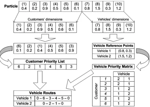
dimension is encoded as a real number. The firstn dimensions are related to customers, each customer is represented by one dimension. The last 2mdimensions are related to vehicles, each vehicle is represented by two dimensions as the reference point in Cartesian map. This solution representation is first proposed byAi and Kachitvichyanukul (2007).
The decoding method for this representation into the CVRP solution starts with extracting the position value of the firstn
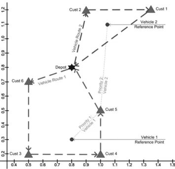
dimension of particle to make a priority list of customer to enter route. It can be done by sorting the firstndimensional values in ascending order and taking the dimension index as the customer priority list. The next step is to extract the reference point for vehicles from the last 2mdimension of particle. The priority ma-trix of vehicles is constructed based on the relative distance be-tween these points and customers location. A customer is prioritized to be served by vehicle which has closer distance. Fi-nally, vehicle routes are constructed based on the customer prior-ity list and vehicle priorprior-ity matrix. The basic procedure of this decoding method is also the same with the decoding method of Ai and Kachitvichyanukul (2007). However, there is a slightly modification in the route construction step, which incorporates 2-opt local improvement procedure to a route right after a cus-tomer is inserted to the route. Schematic example of the whole decoding procedure of the representation SR-1 for problem with 6 customers and 2 vehicles is shown inFig. 1and the route con-struction procedure is graphically illustrated inFig. 2. The nota-tion and the decoding algorithm for this representanota-tion are presented inAlgorithm 2.
Notation
xid Position of theith particle at thedth dimension
Rij Route of thejth vehicle corresponding to theith particle
Algorithm 2. Decoding method of solution representation SR-1
1. Construct the priority list of customers (U). a. Build setS= {1, 2,. . .,n} andU=;.
b. Selectcfrom setSwherexic¼min d2S xid.
c. Addcto the last position in setU. d. Removecfrom setS.
e. Repeat steps 1b–d untilS=;.
2. Construct the vehicle priority matrix (V).
a. Set the vehicle reference position. Forj= 1. . .m, setxrefj=xi,n+j andyrefj=xi,n+m+j.
b. For each customerk,k= 1. . .n.
i. For each vehiclej= 1. . .m, setdjas the Euclidean distance between customerkand the reference point of vehiclej. ii. Build setS= {1, 2,. . .,m} andVk=;.
iii. Selectcfrom setSwheredc¼min d2S dd. iv. Addcto the last position in setVk.
v. Removecfrom setS.
vi. Repeat step 2b.iii–v untilS=;.
3. Construct vehicle route. a. Setk= 1.
b. Add customer one by one to the route. i. Setl=Ukandp= 1.
ii. Setj=Vl,p.
iii. Make a candidate of new route by inserting customerlto the best sequence in the routeRij, which has the smallest additional cost.
iv. Check the capacity and route time constraint of the candi-date route.
v. If a feasible solution is reached, update the routeRijwith the candidate route, then apply 2-opt procedure to the routeRij; go to step 3c.
vi. Ifp=m, go to step 3c. Otherwise, setp=p+ 1 and go to step 3b.ii.
c. Ifk=n, stop. Otherwise, setk=k+ 1 and repeat 3b.
3.2. Solution representation SR-2
The solution representation SR-2 consists of 3m dimensional particle and each particle dimension is encoded as a real number. All dimensions are related to vehicles, each vehicle is represented by three dimensions: two dimensions for the reference point and one dimension for the vehicle coverage radius.
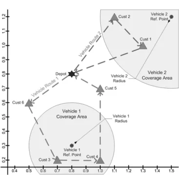
The decoding method for this representation starts with the transformation of particle to the vehicle orientation points and the vehicle coverage radius. The vehicle routes are then con-structed based on these points and radius. For each vehicle, starting from the first to the last vehicle, a feasible route consists of customers that located inside its coverage area and have not been assigned to other vehicle is constructed. Vehicle coverage area is defined as an area inside a circle centered at its reference point within its coverage radius. Afterward, the 2-opt, 1-1 ex-change, and 1-0 exchange procedures are applied to the con-structed routes. If there are remained customers that have not been assigned to any vehicle, the customers are inserted one by one to the existing routes as long as the route feasibility is maintained. Finally, the local improvement procedures are re-ap-plied to all of the routes. Schematic example of the decoding procedure of the representation SR-2 is illustrated inFig. 3 and the route construction procedure is illustrated inFig. 4. The for-mal decoding algorithm for this representation is described in Algorithm 3.
Algorithm 3. Decoding method of solution representation SR-2
1. Extracting vehicle properties, for each vehiclej= 1. . .m. a. Set reference point,xrefj=xi,3j2andyrefj=xi,3j1.
b. Set coverage radius,rj=xi,3j.
2. Route construction.
a. For each vehiclej, construct route of customers that located inside circle with center point (xrefj,yrefj) and radiusrj. Customer is inserted to the route one by one according to its
distance from the center point, priority given to closer customer.
Consider all constraints (vehicle capacity and routing time constraints) to maintaining route feasibility.
Inserting position: best position in the existing route. b. Optimize the partial constructed routes with following local
improvement procedures: 2-opt, 1-1 exchange and 1-0 exchange.
c. For remaining customers, insert to the partial constructed routes:
Customer is inserted to the route one by one according to its distance from the depot, priority is given to customer located further away.
Consider all constraints (vehicle capacity and routing time constraints) to maintaining route feasibility.
Inserting position:
Fig. 2.Illustration of vehicle routes construction of SR-1.
Vehicle: evaluate all, priority given to the closest vehi-cle. Distance of a customer to a route is measured by the distance between the customer to the closest cus-tomer exists in the route.
Customer is inserted before the closest existing cus-tomer in the route.
d. Optimize the routes with the following local improvement procedures: 2-opt, 1-1 exchange and 1-0 exchange.
3.3. Local improvement procedures
Three common local improvement procedures, 2-opt, 1-1 ex-change, and 1-0 exex-change, are incorporated in the decoding meth-ods described in the previous sub section. These procedures will be briefly reviewed in this section.
The 2-opt procedure works on improving single route by systematically exchange the route direction between two pairs of consecutive customers in the route and evaluate whether
the routing cost of the route is improved or not. The exchange mechanism is illustrated in Fig. 5, in which the route direction between customers i(i+ 1) and j(j+ 1) are interchanged. If the routing cost of the modified route is better than the rout-ing cost of original one, the route is updated with the modified one.
The 1-1 exchange and 1-0 exchange procedures work on improving two adjacent routes by exchange customer(s) between routes and evaluate whether the total routing cost of the two routes is improved or not. The 1-1 exchange procedure systemati-cally interchanges one customer from the first route with another customer from the second route. The 1-0 exchange procedure systematically moves one customer from the first route to the second route. If the routing cost of the modified routes is better than the routing cost of original ones, the routes are updated with the modified ones. These procedures are demonstrated inFig. 6 and 7, respectively, in which customeriin the first route is inter-changed with customerjin the second route (Fig. 6) and customer
iin the first route is moved before customerjin the second route (Fig. 7).
The formal algorithm of these local improvement procedures are described inAlgorithms 4–6. In order to reduce the computa-tional effort, an addicomputa-tional step to limit the number of exchange is added to original procedures. In this modified procedures, the exchange is performed whenever the location of customeriandj
are within ranged.
Algorithm 4. Procedure 2-opt
1. Setn= numbers of customer in the route. 2. Fori= 1. . .(n2) andj= (i+ 2). . .n.
a. Modify route by changing the route direction of customer in the sequence numberi, (i+ 1),j, and (j+ 1) as shown inFig. 5. b. Evaluate the feasibility of modified route and the routing cost
improvement.
c. If feasibility is maintained and the routing cost is improved, keep the modified route. Otherwise, return the route to the condition before the last step 2a.
Algorithm 5. Procedure 1-1 exchange
1. Setn= number of customers in the first route. 2. Setm= number of customers in the second route.
Fig. 4.Illustration of vehicle routes construction of SR-2.
Fig. 5.Illustration of 2-opt procedure.
3. Fori= 1. . .nandj= 1. . .m.
a. If the distance between customer with sequence numberiin the first route and customer with sequence numberjin the second route is within ranged, go to step 3b. Otherwise, repeat step 3a with the next value ofiorj.
b. Modify routes by interchanging the customer with sequence numberiin the first route with the customer with sequence numberjin the second route.
c. Evaluate the feasibility of modified routes and the routing cost improvement.
d. If feasibility is maintained and the routing cost is improved, keep the modified route. Otherwise, return the route to the condition before the last step 3a.
Algorithm 6. Procedure 1-0 Exchange
1. Setn= number of customers in the first route. 2. Setm= number of customers in the second route. 3. Fori= 1. . .nandj= 1. . .m.
a. If the distance between customer with sequence numberiin the first route and customer with sequence numberjin the second route is within ranged, go to step 3b. Otherwise, repeat step 3a with the next value ofiorj.
b. Modify routes by moving the customer with sequence number
iin the first route before the customer with sequence numberj
in the second route.
c. Evaluate the feasibility of modified routes and the routing cost improvement.
d. If feasibility is maintained and the routing cost is improved, keep the modified route. Otherwise, return the route to the condition before the last step 3a.
4. Computational result
Two set of computational experiments are conducted to test the performance of the PSO with the two solution representations for solving the CVRP. The first set of experiment is performed in order to compare the result of these proposed methods with PSO ofChen et al. (2006). In this experiment, the proposed methods are applied to the same sixteen benchmark problems that had been used by Chen. The second set of experiment is conducted in order to eval-uate performance of these methods for the larger size problem. The benchmark data set ofChristofides, Mingozzi, and Toth (1979)are selected as testing case, since these data are widely used as CVRP benchmark and they cover larger problems than the Chen’s problem set.
The algorithm is implemented in C# language using Microsoft Visual Studio.NET 1.1 on a PC with Intel P4 3.4 GHz – 1 GB RAM. For each data set, 5 replications of the algorithm are tried. The PSO parameters are: Number of Particle,I= 50; Number of Itera-tion, T= 1000; Number of Neighbor, K= 5; First inertia weight,
w(1) = 0.9; Last inertia weight, w(T) = 0.4; Personal best position acceleration constant, cp= 0.5; Global best position acceleration
constant, cg= 0.5; Local best position acceleration constant,
cl= 1.5; Near neighbor best position acceleration constant,cn= 1.5.
4.1. Comparison with Chen’s results
The first computational experiment is conducted on the same sixteen benchmark problems that had been used by Chen et al. (2006). In these benchmark problems, the total number of custom-ers is varying from 29 to 134 customcustom-ers, and the total number of vehicles is varying from 3 to 10 vehicles. The computational results of both solution representation SR-1 and SR-2 for these benchmark problems are presented in Table 1, in term of the best objective function found and the average computational time over 5 replica-tions. For comparison purpose, the best known solution (BKS) and the Chen’s solution also displayed here. In this table, an objective function value with bold italic typeface indicates that the corre-sponding solution is exactly equal to the best known solution.
From the solution quality point of view, the result from repre-sentation SR-2 is better than Chen’s and SR-1 result. It is shown inTable 1that the SR-2 solutions are very close to the best-known solution, in which the solution of ten out of sixteen instances are exactly same as the best-known solution and the remainders are only slightly larger than the best-known solutions. Furthermore, it provided the best objective function among three methods for al-most all instances (fourteen out of sixteen instances).
In term of computational effort, both representations SR-1 and SR-2 are faster than Chen. Even though the Chen experiment is per-formed on different machines than the SR-1 and SR-2 experiments, the time gap between Chen and SR-1 or SR-2 computational time is significantly large, especially for the big problems, i.e. instance with at least 100 customers (Fn135k7, Mn101k10, etc.). In general, representation SR-1 requires shorter time than SR-2 with
Fig. 7.Illustration of 1-0 exchange procedure.
Table 1
Computational result of the Chen’s benchmark problems
Instance No. cust. No. vhcl. Objective function (Cost) Comp. time (s) BKS Chen SR-1 SR-2 Chenb SR-1 SR-2 An33k5 32 5 661 661a 661a 661a 32 11 13 An46k7 45 7 914 914a 914a 914a 129 19 23 An60k9 59 9 1354 1354a 1366 1355 309 28 40 Bn35k5 34 5 955 955a 955a 955a 38 12 14 Bn45k5 44 5 751 751a 751a 751a 134 17 20 Bn68k9 67 9 1272 1272a 1278 1274 344 33 50 Bn78k10 77 10 1221 1239 1239 1223a 429 41 64 En30k3 29 3 534 534a 541 534a 28 11 16 En51k5 50 5 521 528 521a 521a 301 21 22 En76k7 75 7 682 688 691 682a 527 38 60 Fn72k4 71 4 237 244 237a 237a 398 58 53 Fn135k7 134 7 1162 1215 1184 1162a 1526 178 258 Mn101k10 100 10 820 824 821 820a 874 60 114 Mn121k7 120 7 1034 1038 1041 1036a 1734 88 89 Pn76k4 75 4 593 602 599 594a 496 51 48 Pn101k4 100 4 681 694 686 683a 978 99 86 a
The best objective function among Chen’s, SR-1, and SR-2 results. bComputational time on Pentium IV 1.8 GHz with 256 MB RAM.
exceptions on the instances Fn72k4, Pn76k4 and Pn101k4. These exceptions are not uncommon since the computational effort is also depend on the problem instance characteristics.
As summary, the proposed PSO framework with representation SR-2 can be considered as the best method, since it outperformed SR-1 in terms of solution quality and dominated Chen’s in term of both solution quality and computational time.
4.2. Christofides benchmark problem
The second computational experiment is conducted on the benchmark problems ofChristofides et al. (1979). This benchmark set comprise of problems with randomly distributed and clus-tered customers, problems with and without route time con-straint, and varies number of customers. The computational results for these benchmark problems are presented in Table 2, in term of the best objective function found and the average com-putational time over five replications. For comparison purpose, the best known solution (BKS) and theAi and Kachitvichyanukul’s (2007) results (SR-1°) are also displayed here. In this table, an objective function value with bold italic typeface indicates that the corresponding solution is exactly equal to the best-known solution (BKS) and the value displayed below the solution is the percentage deviation of the solution from the corresponding best-known solution.
The results onTable 2shows that the proposed PSO framework with both representation SR-1 and SR-2 could provide a reasonably good solutions, with an exception for instance vrpnc9 with repre-sentation SR-1. The results for SR-1 are at most within 5.00% devi-ation from the best-known solution and the results for SR-2 are at most within 2.51% deviation from the best-known solution. In addition, one SR-1 solution and four SR-2 solutions are approach-ing exactly the best-known solution. From the computational point of view, it is shown that the representation SR-2 required more computational effort than the SR-1. Also, the computational time
for both representations is reasonable, in which less than four and nine minutes, respectively.
The comparison between the results of representation SR-1° and SR-1 proves that the addition of the local improvement proce-dure in the decoding method has significant effect to the solution quality, since the SR-1 results are generally better than the SR-1° results. Even though this addition causes an additional effort, how-ever, the total computational effort can be reduced by using smal-ler number of particles without affecting the solution quality. The computational results demonstrate that the representation SR-1 using 50 particles is approximately twice faster than the represen-tation SR-1°which was using 100 particles, even if the quality of solution from SR-1 is better than SR-1°.
The high-quality result yielded by the proposed method may come from two factors. First, the decoding scheme gives higher possibility to get feasible solution, since a rigorous constraint checking has already been done while constructing the route. Sec-ond, the solution quality is improved from the route construction heuristics, including the local improvement procedures. The com-binations of these efforts are potential for yielding good solutions.
5. Conclusion
This paper presents two solution representations, 1 and SR-2, and the corresponding decoding methods for solving the capac-itated vehicle routing problem (CVRP) using particle swarm opti-mization (PSO). The representation SR-1 is a (n+ 2m )-dimensional particle for CVRP withncustomers andmvehicles. The representation SR-2 is a 3m-dimensional particle. The pro-posed representations are applied using a framework based on GLNPSO, a PSO algorithm with multiple social learning structures, and tested using some benchmark problems.
The computational result shows that proposed PSO framework with both representation SR-1 and SR-2 is effective for solving CVRP. Both representations are proven more effective than the other PSO method for solving CVRP, in term of solution quality and computational time. In term of solution quality, it is shown that the proposed PSO framework with representation SR-2 is bet-ter than the framework with representation SR-1. However, the representation SR-2 required more computational effort than the representation SR-1.
Some further research for applying the proposed method to other VRP variants should be carried out. Since the variants of VRP differ from one another only on the specific problem con-straints, the adjustment is only required in the constraint feasibil-ity checking of the decoding method. However, the effectiveness of this idea needs further exploration.
Acknowledgements
The authors wish to thank the High Performance Computing Group at Asian Institute of Technology (AITHPC) and the Thai GRID Center for the access of computing facility and the technical support.
The first author expresses gratitude to Universitas Atma Jaya Yogyakarta, Indonesia for providing the financial support for his study in Asian Institute of Technology, Thailand.
References
Ai, T. J., & Kachitvichyanukul, V. (2007). A particle swarm optimization for the capacitated vehicle routing problem.International Journal of Logistics and SCM Systems, 2, 50–55.
Baker, B. M., & Ayechew, M. A. (2003). A genetic algorithm for the vehicle routing problem.Computers & Operations Research, 30, 787–800.
Table 2
Computational result of Christofides benchmark problems Instance No.
cust. No. vhcl.
Objective function (Cost) Comp. time (s) BKS SR-1° SR-1 SR-2 SR-1° SR-1 SR-2 vrpnc1 50 5 524.61 524.61 524.61 524.61a 47 21 24 0.00% 0.00% 0.00% vrpnc2 75 10 835.26 865.86 849.58 844.42a 99 39 57 3.66% 1.71% 1.10% vrpnc3 100 8 826.14 840.91 835.80 829.40a 123 61 101 1.79% 1.17% 0.39% vrpnc4 150 12 1028.42 1068.22 1067.57 1048.89a 235 113 223 3.87% 3.81% 1.99% vrpnc5 199 17 1291.45 1365.15 1345.84 1323.89a 375 188 413 5.72% 4.21% 2.51% vrpnc6 50 6 555.43 560.89 556.68 555.43a 51 21 30 0.98% 0.23% 0.00% vrpnc7 75 11 909.68 – 952.77 917.68a – 42 69 4.74% 0.88% vrpnc8 100 9 865.94 878.59 877.84 867.01a 133 61 115 1.46% 1.37% 0.12% vrpnc9 150 14 1162.55 – N/Ab 1181.14a – 125 295 1.60% vrpnc10 199 18 1395.85 – 1465.66 1428.46a – 208 517 5.00% 2.34% vrpnc11 120 7 1042.11 1045.38 1051.87a 1052.34 133 89 93 0.31% 0.94% 0.98% vrpnc12 100 10 819.56 820.62 820.62 819.56a 128 60 88 0.13% 0.13% 0.00% vrpnc13 120 11 1541.14 1569.14 1566.32 1546.20a 178 86 160 1.84% 1.63% 0.33% vrpnc14 100 11 866.37 866.37 867.13 866.37a 137 64 99 0.00% 0.09% 0.00% a
The best objective function between SR-1 and SR-2 results. b
Berger, J., & Barkaoui, M. (2003). A new hybrid genetic algorithm for the capacitated vehicle routing problem. Journal of the Operational Research Society, 54, 1254–1262.
Bullnheimer, R., Hartl, F., & Strauss, C. (1999). An improved ant system algorithm for the vehicle routing problem.Annals of Operations Research, 89, 319–328.
Chen, A. L., Yang, G. K., & Wu, Z. M. (2006). Hybrid discrete particle swarm optimization algorithm for capacitated vehicle routing problem. Journal of Zhejiang University Science A, 7, 607–614.
Christofides, N., Mingozzi, A., & Toth, P. (1979). The vehicle routing problem. In N. Christofides et al. (Eds.),Combinatorial Optimization(pp. 315–338). Chicester: John Wiley & Sons.
Clerc, M. (2006).Particle Swarm Optimization. London: ISTE.
Cordeau, J. F., Gendreau, M., Laporte, G., Potvin, J. Y., & Semet, F. (2002). A guide to vehicle routing heuristics. Journal of the Operational Research Society, 53, 512–522.
Dantzig, G. B., & Ramser, J. H. (1959). The truck dispatching problem.Management Science, 6, 80–91.
Doerner, K., Gronalt, M., Hartl, R. F., Reimann, M., Strauss, C., & Stummer, M. (2002). Saving ants for the vehicle routing problem. In Cagnoni et al. (Eds.),
EvoWorkshops 2002.LNCS(vol. 2279, pp. 11–20). Berlin: Springer-Verlag. Haimovich, M., Rinnooy Kan, A. H. G., & Stougie, L. (1988). Analysis of heuristics for
vehicle routing problems. In Golden B. L., & Assad, A. A.,Vehicle routing: methods and studies. Amsterdam: North-Holland.
Kennedy, J., & Eberhart, R. (1995). Particle swarm optimization.Proceedings of IEEE International Conference on Neural Networks, 1942–1948.
Kennedy, J., & Eberhart, R. C. (2001).Swarm Intelligence. San Francisco: Morgan Kaufman Publishers.
Lysgaard, J., Letchford, A. N., & Eglese, R. W. (2004). A new branch-and-cut algorithm for the capacitated vehicle routing problem. Mathematical Programming, 100, 423–445.
Pongchairerks, P., & Kachitvichyanukul, V. (2005). A non-homogenous particle swarm optimization with multiple social structures. In Proceedings of international conference on simulation and modeling. A5-02.
Prins, C. (2004). A simple and effective evolutionary algorithm for the vehicle routing problem.Computers & Operations Research, 31, 1985–2002.