MultiObjective Genetic Programming for
Financial Portfolio Management in
Dynamic Environments
Ghada Nasr Aly Hassan
A dissertation submitted in partial fulfillment of the requirements for the degree of
Doctor of Philosophy
of
University College London.
Department of Computer Science University College London
own. Where information has been derived from other sources, I confirm that
this has been indicated in the thesis.
Abstract
Multiobjective (MO) optimisation is a useful technique for evolving portfolio optimisation solutions that span a range from high-return/high-risk to low-return/low-risk. The resulting Pareto front would approximate the risk/reward Efficient Frontier [Mar52], and simplifies the choice of investment model for a given client’s attitude to risk.
However, the financial market is continuously changing and it is essential to ensure that MO solutions are capturing true relationships between financial factors and not merely over fitting the training data. Research on evolutionary algorithms in dynamic environments has been directed towards adapting the algorithm to improve its suitability for retraining whenever a change is detected. Little research focused on how to assess and quantify the success of multiobjective solutions in unseen environments. The multiobjective nature of the problem adds a unique feature to be satisfied to judge robustness of solutions. That is, in addition to examining whether solutions remain optimal in the new environment, we need to ensure that the solutions’ relative positions previously identified on the Pareto front are not altered.
This thesis investigates the performance of Multiobjective Genetic Programming (MOGP) in the dynamic real world problem of portfolio optimisation. The thesis provides new defini-tions and statistical metrics based on phenotypic cluster analysis to quantify robustness of both the solutions and the Pareto front. Focusing on the critical period between an environment change and when retraining occurs, four techniques to improve the robustness of solutions are examined. Namely, the use of a validation data set; diversity preservation; a novel variation on mating restriction; and a combination of both diversity enhancement and mating restriction. In addition, preliminary investigation of using the robustness metrics to quantify the severity of change for optimum tracking in a dynamic portfolio optimisation problem is carried out.
Results show that the techniques used offer statistically significant improvement on the solutions’ robustness, although not on all the robustness criteria simultaneously. Combining the mating restriction with diversity enhancement provided the best robustness results while also greatly enhancing the quality of solutions.
Acknowledgements
I am grateful to my two supervisors, Christopher Clack and Philip Treleaven. This work would not have been possible without their guidance and encouragement. In particular, I have benefited a great deal from working closely with Chris. I believe I was able to improve my research skills through learning from his: reading critically; spotting what is important; and working thoroughly. I am also pretty sure my English has improved through the regular correction of my written texts!
I would like to thank many members of my family, who have given me unconditional support; both emotional and financial. My dear husband has understood the importance of this journey for me, was always there to lift me up, and has willingly made many sacrifices that are only justified by love. My mother took the time and the effort to be in London several times to give very much needed help. My parents in law were tremendously supportive at every step of the way. They all had faith in me, and at some points, more faith than I had in myself. I would not have been able to do it without them, and I will always be indebted to them for this, as well as everything else.
I am very lucky to have come to know many wonderful friends in the 8.11 lab and beyond throughout my stay in London. They made the day-to-day life much more fun and much less lonely. Thank you all for being who you are. I would especially like to acknowledge my dear friend Chi-Chun Chen, who is just an awesome person, my deepest thanks to her for the lovely times, the interesting chats, and the proof-reading!
Last, but certainly not least, my research is funded by a scholarship from the Egyptian government and the Missions program. I am thankful to them for giving me this opportunity. I am also thankful to the Egyptian Cultural Bureau in London for their on-the-ground support, especially the Counsellors Alla El-Gindy, and Amre Abu-Ghazala. I would also like to ac-knowledge Reuters who, through an agreement with my supervisors and UCL, have provided the stock market data used in this research.
Contents
1 Introduction 2 1.1 Motivation . . . 4 1.2 Approach . . . 4 1.3 Problem Statement . . . 5 1.4 Contribution . . . 6 1.5 Thesis Structure . . . 6 1.6 Publications . . . 72 Background and Literature Review 8 2.1 Introduction to Multiobjective Optimisation (MOO) . . . 8
2.1.1 Problem Definition . . . 8
2.1.2 Approaches for Multiobjective optimisation . . . 11
2.2 Multiobjective Evolutionary Algorithms (MOEA) . . . 16
2.2.1 Evolutionary Computation Algorithms . . . 16
2.2.2 State of the Art Multiobjective Evolutionary Algorithms . . . 20
2.2.3 Issues in Multiobjective Evolutionary Algorithms . . . 25
2.3 MOEA in Computational Finance . . . 27
2.3.1 Portfolio Optimisation . . . 27
2.3.2 Stock Ranking and Selection . . . 30
2.3.3 Evolving Trading Rules . . . 31
2.4 Robustness in Dynamic Environments . . . 33
2.4.1 Reliability in Uncertain Environments . . . 33
2.4.2 Stability of Performance . . . 35
2.4.3 Dynamic Optimisation Problems (DOP) . . . 35
2.4.4 Performance Analysis in DOP . . . 42
3 A New Approach for Multiobjective Robustness in Dynamic Environments 45 3.1 Introduction . . . 45
3.2 Critique of existing Multiobjective Robustness Models . . . 47
3.2.1 Terminology . . . 47
Contents vii
3.2.3 Experiment: Performance of an MOGP in a Dynamic Environment . . . . 49
3.3 Problem Analysis and Classification . . . 51
3.3.1 Robustness of an MOGP in a Dynamic Financial Environment . . . 51
3.3.2 What is an Environment Change? . . . 51
3.3.3 Towards an Analysis of Environment Dynamics in the Stock Market . . . 52
3.4 New Approach for Analysis and Assessment of MOGP performance in Dynamic Environments . . . 54
3.4.1 Introduction . . . 54
3.4.2 Definitions . . . 55
3.4.3 Robustness Metrics . . . 56
3.5 Techniques to Enhance MOGP Robustness in Volatile Environments . . . 58
3.5.1 Rank-based Selection Bias . . . 58
3.5.2 Diversity Enhancement . . . 59
3.5.3 Mating Restriction . . . 60
3.6 Optimum Tracking in Dynamic Financial Environments . . . 61
3.6.1 Introduction . . . 61
3.6.2 Proposed Measure for Severity of Change in Dynamic Environments . . . 62
3.7 Summary . . . 62
4 System Architecture and Design of Experiments 64 4.1 Introduction . . . 64
4.2 Real World Problem of Financial Portfolio optimisation with Multiple Objectives 64 4.2.1 Introduction . . . 64
4.2.2 Problem Definition . . . 65
4.2.3 Multiple Objectives of Portfolio optimisation . . . 66
4.2.4 Multifactor Models . . . 68
4.2.5 Measuring Fund Performance . . . 71
4.3 Financial Data and Economic Factors . . . 72
4.3.1 Financial Data Used in Experiments . . . 72
4.3.2 Fundamental and Technical Factors . . . 73
4.3.3 Data Preprocessing . . . 73
4.4 System Architecture . . . 75
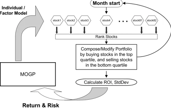
4.4.1 The Investment Simulator . . . 75
4.4.2 The Multiobjective GP . . . 78
4.5 Performance Analysis . . . 80
4.5.1 MOGP Performance in Training . . . 80
4.5.2 Portfolio Performance in Training and Validation . . . 82
4.5.3 Robustness of Solutions and the Pareto Front in Validation . . . 83
4.6 Notes on Design and Implementation of Experiments . . . 85
4.6.1 Data Normalisation . . . 85
4.6.2 Guarding Against Bias . . . 85
4.6.3 Clustering of Solutions . . . 86
4.6.4 Ranking Solutions . . . 86
4.6.5 GP Diversity . . . 87
5 Experiments and Results 89 5.1 Performance Benchmarks . . . 89
5.1.1 Buy–and–Hold Strategy: Index–Fund . . . 90
5.1.2 Random Strategies: Lottery–Trading . . . 91
5.1.3 Pareto Front Metrics . . . 93
5.2 Suitability of MOGP for Portfolio Optimization . . . 93
5.2.1 Performance in Training: Stability . . . 93
5.2.2 Performance in Training: Quality . . . 94
5.3 MOGP Robustness: Performance on Unseen Data . . . 96
5.3.1 Investment Performance against Benchmarks . . . 98
5.3.2 Pareto Front Performance . . . 101
5.3.3 Selection Bias Effect on Robustness of MOEA . . . 102
5.3.4 Diversity and Cluster-Based Mating Restriction for MOEA Improved Ro-bustness in a Financial Dynamic Environment . . . 106
5.3.5 Summary and Discussion . . . 111
5.4 Optimum Tracking, Change Detection, and Analysis of Market Behaviour . . . . 111
5.4.1 Severity of Change in Dynamic Environments . . . 111
5.4.2 Preliminary Analysis of Factors Selected in Models Evolved by MOGP . . 118
6 Discussion and Conclusion 128 6.1 Robustness in Multiobjective Optimization . . . 128
6.2 Portfolio Management Using MOGP . . . 131
6.3 Summary and Conclusion . . . 132
6.4 Future Research . . . 133
6.5 Contributions . . . 133
Appendices 134
A Sample MOGP Factor Models 135
List of Figures
2.1 Optimisation Trade-offand Pareto Optimality . . . 10
2.2 Convex Pareto Front. Each Point on the front is a stable minimum corresponding to a given weight combination (A rotation angle) . . . 12
2.3 A concave Pareto front. Only the two points at the two ends of the front are stable minima . . . 12
2.4 Basic Evolutionary Algorithms Life Cycle . . . 16
2.5 Sample Genetic Programming Tree Structure . . . 18
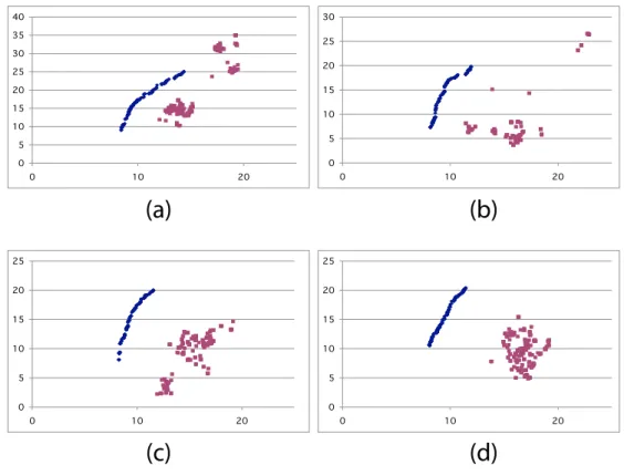
3.1 SPEA2 Pareto Fronts in Training (blue, upper left) and Validation (red, lower right) over four runs. The x-axis is risk, and y-axis is return . . . 49
3.2 Example of Solutions Changing their Objectives Profile(Cluster). The vertical axis is return on investment, and the horizontal axis measures risk. The x-axis is risk, and y-axis is return . . . 50
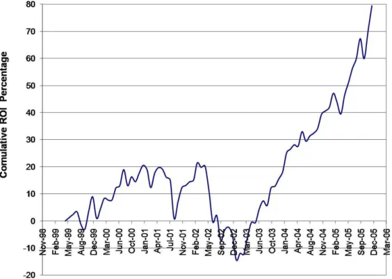
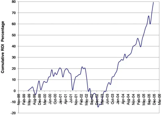
3.3 Performance of Index Fund Benchmark . . . 53
4.1 Efficient frontier in standard-deviation, expected-return space . . . 66
4.2 System Architecture . . . 76
4.3 Classification of solutions into clusters — a robust system is one where solutions do not change clusters as the environment changes . . . 86
4.4 Ranking of solutions — a robust system is one where solutionsminimallychange their relative rank with respect to other solutions . . . 86
5.1 Performance of Index Fund Benchmark . . . 90
5.2 Pareto fronts for training on Months May1999-December2000 . . . 95
5.3 Pareto fronts for training on Months January2001-August2002 . . . 95
5.4 Pareto fronts for training on Months September2002-April2004 . . . 95
5.5 Pareto fronts for training on Months May2004-December2005 . . . 95
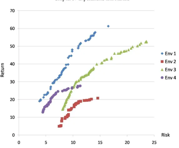
5.6 Approximation of the True Pareto Fronts in the Four Environments . . . 96
5.7 SPEA2 Pareto Fronts in Training (black) and Validation (grey) over four runs – x-axis is Risk and y-axis is Return . . . 101
5.8 Example of Solutions Changing their Objectives Profile(Cluster). The vertical axis measures return (percentage return on investment), and the horizontal axis
measures risk (standard deviation of monthly returns). . . 102
5.9 Performance of Index Fund During Training Period . . . 104
5.10 Performance of Index Fund During Validation Period . . . 120
5.11 R-SPEA2 Performance in Training (black) and Validation (grey) over four runs. The vertical axis measures return (percentage return on investment), and the horizontal axis measures risk (standard deviation of monthly returns) . . . 120
5.12 Sharpe and Sortino Ratios . . . 121
5.13 Points Changing Cluster . . . 121
5.14 Average Distance Cluster Change . . . 122
5.15 Spearman Correlation Coefficient . . . 122
5.16 The HRS and Spread Metrics . . . 123
5.17 Market Index Return on Investment (ROI) . . . 123
5.18 The Efficient Frontier in each of the Four Environments . . . 124
5.19 Performance of archive solutions evolved in Env1 when Env2 is introduced . . . 124
5.20 Performance of archive solutions evolved in Env1 when Env3 is introduced . . . 125
5.21 Performance of archive solutions evolved in Env1 when Env4 is introduced . . . 125
5.22 Retraining every 5 months (moving window) — previous vs. random popula-tion. With standard deviations. . . 126
5.23 Retraining every 20 months (fresh data) — previous vs. random population. With standard deviations. . . 126
5.24 Histogram of Factors used in Investment Strategies Evolved - The y-axis indicates number of runs out of 10 . . . 127
List of Tables
3.1 Cluster Distance Change Measurement . . . 56
4.1 Definition of Financial and Economic Factors Used . . . 74
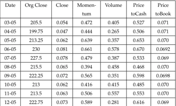
4.2 A sample of Company Data (BT) . . . 75
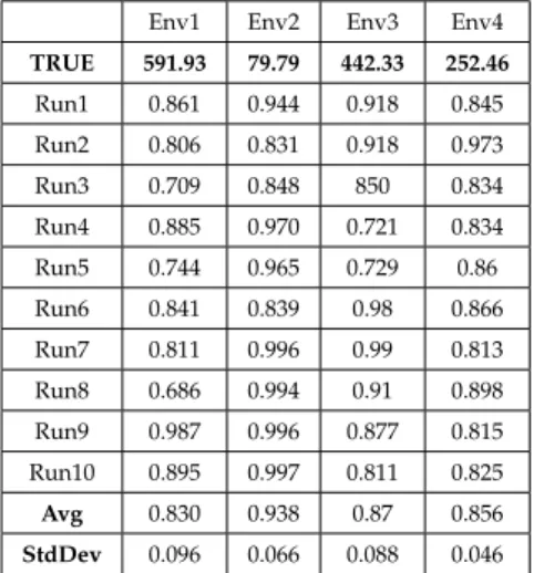
5.1 Size of the space dominated by the fronts and the Hypervolume ratio of each (in comparison to the hypothetical true front) . . . 97
5.2 Spread characteristics of the fronts in the four environments . . . 97
5.3 MOGP Performance in Training against Index–Fund (IF) and Lottery–Trading (LT) over the four environments . . . 98
5.4 Index–Fund Performance on the 4 Environments . . . 98
5.5 Validation Performance of Training on Env1 . . . 99
5.6 Validation Performance of Training on Env2 . . . 99
5.7 Validation Performance of Training on Env3 . . . 99
5.8 Validation Performance of Training on Env4 . . . 99
5.9 Mean distance of cluster change and percentage number of solutions changing cluster for SPEA2 and R-SPEA2 . . . 105
5.10 Correlating between Training and Validation: Spearman Coefficients of Objectives105 5.11 Statistical Test Results (Validation) . . . 111
5.12 Raw (Normalised) Distance Between Cluster Centroids as a Proxy for Change in Location and Shape of Front. Lower values are better. . . 114
5.13 Shuffle: The Correlation between Solutions Ranks on Both Objectives a Proxy for Severity of Change. Higher values are better. . . 114
Introduction
In the field of computational finance, Machine Learning (ML) and Artificial Intelligence (AI) algorithms and techniques are often used to investigate problems in the area of finance and eco-nomics. Machine Learning algorithms are distinguished by their capability for mechanical self improvement through experience, as evident in the Neural Network (NN) learning algorithms, Evolutionary Algorithms (EA), Decision Trees and Reinforcement Learning. The flourishing computational finance field owes its success to the current advances in computing in both algorithms and hardware; more data on financial systems is becoming available; algorithms suitable for deeper analysis of data are being developed; the processing power of computer hardware is accelerating; and memory storage capacity is of much less concern now than it used to be. These factors are enabling researchers to analyse the complex financial and economical models better, helping them to gain more insight into the dynamics governing the financial market and assist the decision-making process based on the new knowledge acquired. There are a number of financial areas in which machine learning algorithms have been applied, such as [TMJ04]: forecasting financial time series, exploiting arbitrage opportunities, challenging the fundamentals of finance and economics, and portfolio selection and management.
This thesis focuses on evolving rules for stock selection in a portfolio management problem. In the early conventional view of investment and trading, optimisation methods and trading strategies often assumed return maximisation as the sole objective of the investor, and as the only performance measure. The introduction of the Markowitz mean-variance approach [Mar52], brought to light ‘risk’ (to be minimised) as another objective of the rational investor and emphasised the concept of selecting a portfolio of investment assets which collectively have lower risk than any single individual asset therein. Markowitz described the portfolio optimisation problem as a problem of optimising two contradicting objectives of risk and return, and the problem came to be recognised as a multiobjective (MO) one. Recently, it is increasingly acknowledged that investors may actually have, in addition, more objectives that they would like their investment to fulfil. Examples of such objectives are portfolio liquidity, various measures of risk, dividend return, growth in sales, and amount invested in R&D, as shown in [CAS04] and [SQ05].
3
The recognition of multiobjective optimization problems in finance, and using MOEA to solve them is a recent development. Examples of applying MOEA in financial applications1
include: risk management [SMS05], bank loan management [MBDM02] as well as management of financial portfolios [AL05, LT06, SBE+05, Lau05, MERTS06, SKN07].
Existing research reveals successes as well as problems and gaps. Some are specific to the financial domain but others are inherent in the multiobjective algorithms. One of these problems is the performance and applicability of MO algorithms when the environment is changing. We call this problem ‘robustness in dynamic environments’ and it deals with two aspects of multiobjective optimization. The first of these is how to examine and improve the performance of the multiobjective solutions on out-of-sample environments. Secondly, it is concerned with how to measure the degree of environment change beyond which the algorithm will need to be modified or retrained to adapt to the changing environment. Robustness isnot a requirementin a stationary environment, where the problem at hand has its environment fixed by definition; that is to say optimisation problems in which the range and behaviour of the input data is known and fixed, and the optimization algorithm task is to find solutions that will yield the best tradeoffs between objectives once and for all. Robustness isdesirablewhen the change in the environment is small due to noise in the input decision variables or the uncertainty of objectives. However, when the optimization problem has a continuously changing environment by nature, then investigating robustness becomes animportantrequirement.
What concerns this research in particular is the correlation between the time series data that are available to the stock-picking model in training and the future performance of the rules evolved based on available data. Our stock-picking models do not have to predict precise future stock prices, but they are required to rank the stocks correctly based on establishing a relationship between their historical fundamental/technical factors and the stock’s future performance. If the correlation between time series and future stock performance changes, then a given model (equation) may become less effective in ranking stocks. Previous work on multiobjective GP [LT06] and single objective GP [YC06] have shown that the performance of MOGP and GP evolved stock-picking equations can vary substantially when used in an out-of-sample-environment. However, all previous studies have only considered optimality (as measured by one or another financial related measure for investment success). In the case of a single objective GP, the output is one solution, and the optimality of this solution on out-of-sample environments is often used as measure of the robustness of the algorithm [Kab00, PSV04, YC06]. In the case of multiobjective GP, and since the output is a set of solutions, the average performance of the solution set is sometimes taken as the measure of performance on the out-of-sample environment as in [Bin07, BFF07, BJ08], and hence the robustness of the algorithm. In practice, however, investment will be carried out using individual rules from the solution set. The individual solutions will be selected based on the client’s appetite for risk,
and in return his expectation of a certain degree of profit. Hence, in addition to optimality on the out-of-sample environment, a practitioner will be equally interested in ensuring that the perceived relative positions of solutions on the Pareto front do not switch (for example a situation where a “lowest-risk” portfolio becomes “highest-risk”).
1.1 Motivation
Robustness of MOGP solutions is extremely important for the real-world problem of stock-picking for a monthly investment portfolio. It is therefore essential for MOGP solutions to be analysed inunseenenvironments, not just in training, and although it may be difficult to define an absolute measure of solution robustness we must be able to determine which of two solutions is more robust, and which of two Pareto fronts is more robust.
The motivation for this research is the investigation of the effectiveness of a multiobjective genetic programming approach, to evolve robust factor models for stock ranking, in a real world portfolio management problem. The MOGP evolved Pareto front accurately depicts the tradeoffbetween risk and return in training (although the real Pareto front is generally not known). To ensure the practical utility of such an algorithm, the robustness of solutions in subsequent unseen (test) environment is examined.
In volatile environments such as the financial markets, robustness is of major importance. If robustness is not achieved, the solutions will exhibit unstable performance that may render them unfit in subsequent environments, and the algorithm is only useful as an analysis tool of historical data. Investors ideally prefer a solution whose specific risk and return never changes. Given that this is highly unlikely ever to be achieved in a volatile market, the next best solution is one that sustains the characteristics of its objectives. For example, given a solution with the lowest risk relative to the available alternative solutions, it should continue to give the lowest relative risk as the environment changes (even though the precise objective value of risk may change). This aspect of robustness performance of the MO algorithms has not previously been identified. We believe that this particular aspect is as important as optimality when it comes to the practicality of using MO solutions in real life optimization problems.
1.2 Approach
So how should the system respond to market instability? One obvious response is to employ dynamic adaptation via retraining, using new training data drawn from the new environments. However, in the context of monthly investment this is problematic:
• The most pressing problem is the lack of new data, because the time series comprises only monthly data — it is not feasible to train on just a handful of data points, so the system must wait many months before sufficient new data has been gathered to permit retraining (and by that time, the market may have changed again);
1.3. Problem Statement 5
where it continuously retrains on the most recent (say) twelve months of data — the disadvantage with this approach is that for the first (say) six months following a change the training data will predominantly come from the old environment, and so it will still take considerable time before more suitable equations can be evolved;
• How often should the system retrain? Too frequently, and too little data will be available; too infrequently, and the retraining may be ineffective because it happens at the wrong time (for example, just before a change in the market);
• Should the system only retrain when a change in the market trend is detected? This would appear to be a better solution, but turns out to be difficult to achieve, as explained below.
Certain gross behaviour of the financial markets (for example, a “bull”, “bear”, or “volatile” market) can be identified by inspection of the behaviour of a benchmark portfolio (or “index” portfolio) which invests in all stocks equally (alternatively, investing in all stocks using a standard weighting such as capitalisation). The index can therefore be used to identify a change in market environment. However, it turns out to be very difficult to detect the point at which a market changes — it is relatively easy to identify a “bull” or a “bear” market once it is established, but at the turning point it can be difficult to know for certain whether the market is really changing, and difficult to determine the nature of the new market (is it changing from “bull” to “bear” or from “bull” to “volatile”?).
1.3 Problem Statement
Despite the broad range of research in MO algorithms, most of this work has focused on static optimisation and hence on generating solutions on the Pareto front that are diverse and well-distributed. Little attention has been paid to therobustnessof solutions evolved in dynamic environments, and they are not always validated in out-of-sample environments. When MO algorithms are used for dynamic optimisation, two issues arise: the performance of the solutions found in training when used in new environments, and the ability of the algorithm to continuously adapt to changing environments.
Whilst retraining is an important tool in responding to the instability of the markets it is insufficient on its own; it is also necessary to ensure that the evolved models will continue to performreasonablywell when the market environment in which they are used is different to that in which they were trained. We do not expect them to continue to behave well but we can require that they degrade gracefully within a range of market change and do not suddenly produce catastrophically wrong results (it would be unreasonable to expect good behaviour for a sudden extreme change). We call this “solution robustness” and it is important because it provides a period of time within which either new data can be gathered for retraining or human intervention can take over prior to retraining.
The aim of this research is to investigate the robustness of MOGP solutions to the multi objective real world problem of portfolio management. We achieve this objective through introducing new definitions and metrics for robustness in the multiobjective context, and developing techniques for improving robustness of solutions on the Pareto front. We also provide preliminary results on quantifying change in the stock market environments for which solutions are no longer valid and re-optimization is required.
1.4 Contribution
This thesis provides an empirical study of using an MOGP to evolve robust non-linear factor models for stock selection in a portfolio optimization problem with multiple objectives, and an assessment of the performance/robustness of the MOGP solutions when applied to out-of-sample data. It also demonstrates the value of an MOGP approach to a finance practitioner. The thesis makes the following contributions:
1. The development of new definitions and metrics for the robustness of MOGP solutions and robustness of the Pareto fronts in dynamic environments.
2. The use of the new definitions and metrics to assess the effect on robustness in unseen environments of:
(a) Selection bias.
(b) Diversity preservation.
(c) Cluster-based mating restriction. 3. A preliminary analysis of:
(a) The Dynamics of change.
(b) How to quantify the severity of change in the financial environments. (c) The use of MOGP as an analysis tool in the financial market.
1.5 Thesis Structure
The rest of the thesis is organised as follows:
• In Chapter 2, background information is provided on genetic computation, and multi-objective optimization concepts, followed by some of the best known MOEAs, then a survey of applications of MOEA in finance and a survey on the related literature on robustness of MO algorithms.
• Chapter 3 provides a critical analysis of the current state of the art in robustness of MO algorithms, followed by suggestions for a new model for robustness.
1.6. Publications 7
• Chapter 5 provides results of experiments on the robustness of multiobjective genetic programming for portfolio management.
• Chapter 6 presents a discussion and conclusions on the implications of results on ro-bustness of MOGP as well as on the practical use of MOGP in real world portfolio optimization.
1.6 Publications
• G.Hassan and C.Clack. Multiobjective Robustness for Portfolio Optimization in Volatile Environments. GECCO’08: Proceedings of the 10th Annual Conference on Genetic and Evolutionary Computation, pages 1507-1514, Atlanta, GA, USA, 2008. ACM. (Nominated for a best paper award).
• G.Hassan. Non-Linear Factor Model for Asset Selection using Multi Objective Genetic Programming. GECCO’08 Workshop: Advanced Research Challenges in Financial Evo-lutionary Computing (ARC-FEC), pages 1859-1862, Atlanta, GA, USA, 2008. ACM.
• G.Hassan and C.Clack. ”Robustness of Multiobjective GP Stock-picking in Unstable Financial Markets”. GECCO’09: Proceedings of the 11th Annual Conference on Genetic and Evolutionary Computation, pages 1513-1520, Montreal, 2009. ACM.
• G.Hassan and C.Clack. ”Dynamic Multiobjective Optimization for Optimum Tracking in Portfolio Optimisation”. Submitted for GECCO’10: Proceedings of the 12th Annual Conference on Genetic and Evolutionary Computation.
Background and Literature Review
This chapter presents background information and reviews existing literature that is relevant to the work in this thesis. The chapter is divided into four main sections:
• Section 2.1 gives the formal definition of multiobjective optimisation problems, and out-lines the various approaches for solving them.
• Section 2.2 concentrates on one of those approaches: the multiobjective evolutionary algorithms (MOEA) . It explains the state of the art algorithms belonging to this approach and briefly presents some of the research challenges they currently face.
• Section 2.3 presents a sample of the research on using MOEA in a range of problems from economics and finance.
• Section 2.4 reviews the existing literature on robustness of MOEA, specifically the research on their application in dynamic environments.
2.1 Introduction to Multiobjective Optimisation (MOO)
Multiobjective optimisation is the problem of finding the best solution to an optimisation problem with more one than objective. In this section we first give the formal definition to the problem in Section 2.1.1, and discuss in section 2.1.2 the different solution approaches in the literature. We review the weighted aggregation, multiple populations, Pareto dominance, and alternatives to the Pareto dominance approaches.
2.1.1 Problem Definition
Optimisation refers to the problem of finding the best solution to a problem given a set of inputs and constraints [Coe05b]. In its simpler variety, the single objective optimisation, there is a sin-gle objective to be minimised or maximised. The solution to the problem is a global optimum in the search space (as represented by the function that we seek to optimise). However, in many problems, it is usually the case that we seek to optimise a number of – often conflicting– objectives. When the problem seeks to optimise two or more objectives, it is known as multiob-jective, and may require different algorithms and tools than those used in the single objective
2.1. Introduction to Multiobjective Optimisation (MOO) 9
optimisation problem [Coe05b, FA02]. In multiobjective optimisation, and when the objectives are conflicting, a single solution that can optimise all objectives simultaneously does not exist. Hence, the goal of the search is to produce a set of“trade-offs” between different objectives. The most common notion of optimality to express this trade-off is that proposed by Francis Edgeworth and generalized by Vilfredo Pareto, hence known as Edgeworth-Pareto optimality or often just Pareto optimality. The traditional methods for dealing with the single-objective and multiobjective optimisation problems are sound in the research in the mathematical field of operations research and mathematical programming. Mathematically, an optimisation problem has the following form [CS03]:
minimise f(x) (function to be optimised) withgi(x)≥0 (m inequality constraints)
andhi(x)=0 (p equality constraints) Definition 1. Objective Function
The name given to the function f. It is the function for which the algorithm will try to find its optimal value. In multiobjective problems there are multiple objective functions to be optimised.
Definition 2. Decision Variables
Consider a search spaceΩwithnparameters, these parameters are called the decision variables, and they are the values taken by the vectorx =[x1,x2,x3, ...,xn]T. It is by changing this vector
that we are searching for the optimal through traversing the search spaceΩ.
Definition 3. Global Minimum
In single objective minimisation problems, the global minimum is the optimal result of the search algorithm. The vectorx∗ is global minimum of the function f if f(x∗) ≤ f(x) for any
x∈Ω.
Definition 4. The Multiobjective Problem
In mutliobjective problems, for each point in the search space there are mdifferent criteria by which to judge that point. The multiobjective optimisation problem is to find the value of decision variables forx∗ = [x∗
1,x∗2, . . . ,x∗n]T, from total set of vectors in the search spaceΩthat
will be a solution to:
F(x)=[f1(x),f2(x), . . . ,fk(x)], wherekis the number of objective functions
subject to theminequality constraintsgi(x)≥0, fori=1,2, . . . ,m,
and thepequality constraintshi(x)=0, fori=1,2, . . . ,p Definition 5. Pareto Dominance
A solution vector x = [x1,x2,x3, ...,xn]T is said to dominate another solution vector v =
minimisation is required):
xv i f f :
fi(x)≤ fi(v) for all i∈[1,2, ...,k],and
fj(x)< fj(v) for at least one j∈[1,2, ...,k]
(2.1)
Definition 6. Pareto Optimality
A solutionx∗ is said to be Pareto optimal in the search spaceΩ if there is no solutionvfor
whichvx∗
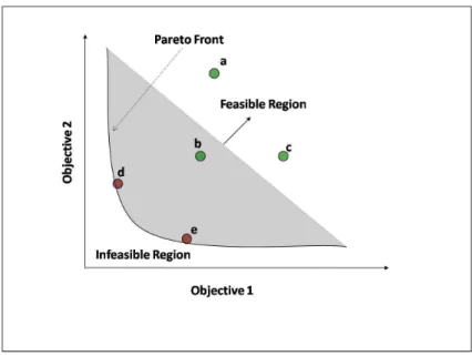
This definition says that a vector is Pareto optimal if there exists no other vector of decision variables belonging to the feasible set of solutions that would improve some decision criterion without deterioration in at least one other criterion. This definition always gives a set of solution vectors called the Pareto optimal set (see below). The solution vectors in the set are called non-dominated in the sense that no other solution is better (dominates them). The plot in the value space of the objective functions whose non-dominated vectors constitute the Pareto optimal set is called the Pareto front (see below), as shown in Figure 2.1, where the points a,b,c,d,e lie in the feasible region of the search space, and the point d,e lie on the Pareto front as they are non-dominated by any other points in the feasible region of the space.
Figure 2.1: Optimisation Trade-offand Pareto Optimality
Definition 7. Pareto Optimal Set
For a given multiobjective problem, the Pareto optimal set is defined as:
P∗=x∈Ω|@v∈Ω:F(v)F(x) (2.2)
Definition 8. Pareto Front
2.1. Introduction to Multiobjective Optimisation (MOO) 11
PF∗=F(x)= f
1(x),f2(x), ...,fn(x)|x∈P∗ (2.3)
2.1.2 Approaches for Multiobjective optimisation
In this section, we provide an overview of four different approaches to multiobjective optimisa-tion problems: weighted aggregaoptimisa-tion; populaoptimisa-tion approach; Pareto optimality; and alternatives to Pareto optimality.
2.1.2.1 Weighted Aggregation Approach
The intuitive way to solve the multiobjective problem is by weighted aggregation. In this approach, different objectives are weighted and combined in one single objective [LT99]. The weights are non-negative and are usually fixed during optimisation.
Effectively, using weighted aggregation ignores the multiobjective nature of the problem and attempts to solve it as a single objective one. The transformation is achieved through defining another objective f∗, equivalent to the aggregated function of the original objectives
(f2,f2,f3, ...,fk). When integrated within an evolutionary algorithm, the fitness function of the
evolutionary algorithm is defined to be this weighted aggregation of objectives. So, for example, the fitness function of a two objective (f1,f2) problem will be defined as:
f∗=w
1f1+w2f2, wherew1+w2=1
Examples of using the weighted aggregation approach as the fitness function within an evolu-tionary algorithm are found in [JGSB92, SP91].
The weighted aggregation method is easy to understand and implement. However, the method will yield a single solution for every combination of weights used in any one single run. It is also quite impossible to know the correct weights to generate points evenly distributed along the Pareto front if we do not know its exact shape, as discussed and analysed in [DD97]. In addition, the weighted aggregation method will only be able to find the solutions if the Pareto front is convex. Otherwise, if the Pareto front is non-convex, the solutions cannot be found using weighted aggregation.
A Note on Weighted–Sum Optimisation on Convex and Concave Fronts
This note is based on [YOS01], in which the authors offer an explanation of why the non-convex Pareto front poses problems for weighted-aggregation optimisation. In [DD97] the author also gives a similar explanation using geometry and the characteristics of tangents to convex and concave functions to explain why solutions on the concave regions of the Pareto front cannot be obtained by weighted aggregation. In [YOS01], Jin et. al explain why their Evolutionary Dynamic Weighted Aggregation (EDWA) overcomes the difficulties encountered with a Fixed Conventional Weighted Aggregation (CWA).
Definition 9. Convex Pareto Set
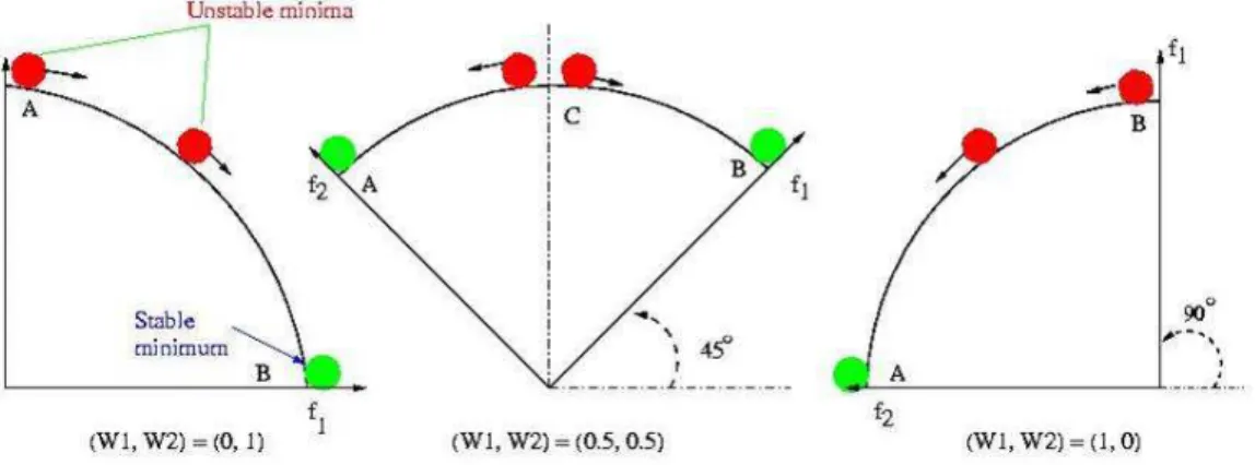
Figure 2.2: Convex Pareto Front. Each Point on the front is a stable minimum corresponding to a given weight combination (A rotation angle)
every point on the segment that links these two points liein S[CS03].
Definition 10.Concave Pareto Set
A set of pointsSin the Euclidean space is concave if, given any two distinct points in the set, every point on the segment linking these two points lieoutside S[CS03].
Figure 2.3: A concave Pareto front. Only the two points at the two ends of the front are stable minima
As the authors explain, the CWA is able to converge to a Pareto optimal solution if the Pareto solution corresponding to a given weight combination is a stable minimum. For the two-objective problem presented in Figure 2.2 (in the first graph to the left), pointBis the stable minimum and will be the point that the algorithm converges to, given the weight combination (w1,w2)=(0,1). If the weight combination is changed, it is equivalent to rotating the coordinate
system together with the Pareto front. Hence, when w1 decreases and w2 increases, it can
be represented as the rotation of the coordinate system counter clockwise. For the weight combination (w1,w2)=(0.5,0.5), the coordinate system rotates 45 degrees, as shown in Figure
2.2 (middle graph), and the pointCbecomes the stable minimum. using the same principal, it becomes clear that in the case of a convex Pareto front, each weight combination corresponds to
2.1. Introduction to Multiobjective Optimisation (MOO) 13
a stable minimum on the Pareto front. Changing the weights will cause the optimiser to move from one stable minimum to another. As the weights are non-negative, the maximal rotation angle is 90 degrees at which the stable minimum is pointA.
For a concave Pareto front, all solutions with exception of the two points on the two ends are unstable minima, see Figure 2.3. At a 0 degrees rotation angle, the stable minimum is pointB. For all weight combinations corresponding to a rotation between 0 and 45 degrees, the solution obtained will be point B. Whereas for all weight combinations corresponding to rotations between 45 and 90 degrees, the solution will be pointA. In the case of a weight combination of (w1,w2)=(0.5,0.5) corresponding to the rotation 45 degrees, the weight combination will be
a dividing point, and the result of the optimisation will be eitherAorB. As a conclusion, the authors state that a weighted aggregation optimisation algorithm will only converge to either of the two points whatever weight combination is used.
To overcome some of the mentioned problems, an approach called “Dynamic Weighted Aggregation” is proposed in [YOS01] where weights are attached to objectives and are allowed to change dynamically during the evolution process. The authors use an evolutionary strategy algorithm, which proceeds as usual with fitness assignment and reproduction. However, the algorithm seeks to find the points of the Pareto front as it is going along, and the weights for the different objectives are set dynamically, then are gradually and periodically changed during optimisation. Whenever a new non-dominated solution is found, it is archived, and in this way, the whole Pareto front is archived. For a two-objective problem, the weights are defined as:
w1(t)=|sin(2πFt)| , and
w2(t)=1−w1(t)
wheretis the generation number andFis a constant that adjusts the frequency of changing the weights. Since the population will not be able to keep all the found Pareto solutions, an archive is used to keep the non-dominated solutions that are found. The method is tested on a range of multiobjective optimisation problems; with both convex and concave, as well as continuous and discontinuous, Pareto fronts .
This method overcomes some of the problems of fixed weighted aggregation. There is no need to decide on the weights a priori, we can obtain the Pareto solutions in one run and it is able to find solutions on the concave regions of the Pareto front as well as the convex. The reason for this, as the author explains, is that although on a concave front only two solutions corresponding to two weights are stable, all of the points of the front are reachable. He uses this fact, and does not force the algorithm to converge to one global minimum, but rather search for non-dominated solutions, which when found, are extracted from the population and added to the solution set.
Consequently, the actual technique for finding the Pareto optimal solutions is the archive maintenance and not the result of the evolutionary optimisation algorithm. The archive main-tenance algorithm looks at each offspring generated and tests whether it is non-dominated by
members of the population as well as members of the archive. If this is the case, it adds it on to the archive. On the evolutionary algorithm side, and by continuously changing the weights and hence the fitness function, the EA is not being pressed to converge to any particular area but is merely used as a mechanism for traversing the space.
2.1.2.2 Population Approach
The Vector Evaluated Genetic Algorithm (VEGA) was proposed by Shaffer [Sch85]. The al-gorithm starts by randomly initialising a population as in standard GA, then divides it into a number of sub-populations equivalent to the number of objectives. Then, each sub-population’s individuals are rated and selected according to one of the objectives, and hence, this particular subpopulation is pushed to evolve towards this one objective. Afterwards, the selected indi-viduals are shuffled and allowed to reproduce as usual. The problem inherent in the algorithm was realised by Schaffer himself. He called it “middling”. Since the algorithm looks at each sub-population with regard to only one objective and hence chooses individuals that excel in this specific criterion, we are deliberately ignoring individuals that may not be the best in any single criterion but offer a good compromise solution between all criteria.
In another population approach used in [KCV02], the Cooperative Co-evolutionary Al-gorithm [MAP95] was used to evolve subpopulations to solve the multiobjective optimisation problem. The approach proposed an integration between MOGA [FF93b] (see Section 2.2.2.5) and a Cooperative Co-evolutionary Genetic Algorithm (CCGA). Similar to the CCGA, each species in the MOCCGA represents a decision variable or a part of the problem that needs to be optimised. However, instead of directly assigning a fitness value to the individual of interest which participates in the construction of the complete solution, a rank value will be determined first. Similar to the MOGA, the rank of each individual will be obtained after comparing it with the remaining individuals from the same species on all the objectives. Then a fitness value can be interpolated onto the individual where a standard genetic algorithm can be applied within each sub-population. The algorithm was compared to MOGA, and the authors found that the number of non-dominated solutions found is higher and the coverage of the front is better in the case of MOCCGA.
Authors of [IL04] used a Cooperative Co-evolutionary Genetic Algorithm in which n– subpopulations are created randomly corresponding to thendecision variables to be optimised, and each is responsible for a decision variablexi. In evaluation of individuals from the first
generation, random individuals from the subpopulations collaborate and are evaluated on the objectives. The result of the evaluation is assigned as the fitness of the individual undergoing evaluation. In subsequent generations, an individual is evaluated by collaboration with a randomly selected component from the best non-domination levels in the previous generation subpopulation. Then both the parents and the children are sorted according to their domination information and the worst individuals are deleted, maintaining a constant population size. Tournament selection is used to select individuals for mating such that a solutioniwins the
2.1. Introduction to Multiobjective Optimisation (MOO) 15
tournament against solution jif: it has a better domination level, or, in the case of bothiand j
having the same domination level, ifihas a better crowding distance thanj. The algorithm was found to produce comparable results to that of NSGAII (see section 2.2.2.4) on some problems. Population approaches rely on the creation of subpopulations where each is responsible for optimising on of the objective functions, and they collaborate to achieve the required objectives. However, this class of algorithms can only deal with problems where distinct and separate components of a solution can be identified. Real world problems, where the variables are highly correlated, create a real difficulty for these algorithms and may cause its performance to deteriorate.
2.1.2.3 Pareto Optimality (PO) Approach
These algorithms are characterised by their use of the dominance concept to differentiate between solutions in the search space, and to eventually arrive at a set of solutions as close as possible to the Pareto optimal set1.
The major advantage of the Pareto optimality approach is that it gives a large number of alternative solutions near the Pareto front in one single run. The assumption is that the decision maker will be given these solutions, out of which he will choose the most suitable. In Section 2.2, we review some of the existing multiobjective evolutionary algorithms that utilise Pareto optimality concepts.
2.1.2.4 Alternatives to Pareto Dominance
[DDB01, SDGD01] define the relationship “Preferred”, in which a solution A is said to be preferred toB, if it is better than B in a larger number of objectives than Bis better thanA. This is in contrast to the relationship “Dominates”, whereAis said to dominateBif it is better than or equal toBin all objectives but is strictly better in at least one objective. The algorithm builds strongly-connected components in the relationship graph that result from the pair-wise comparison of all individuals of the population. All individuals in the same component obtain the same fitness. Then all components are hierarchically ordered followed by assignment of ranking values.
Kukkonen and Lampinen in [KL07] suggest ranking solutions according to each separate objective and the use of an aggregation function that results in a scalar fitness value for each solution to enable the sorting of solutions in the case of a large number of objectives. The aggre-gation functions suggested are Sum, and Minimum. The complexity of ranking isO(MNlogN). Results of comparing this method to the Pareto dominance were reported on the test suite DTLZ 1-6 [DTLZ02]. The authors found that on problems (DTLZ 1-4) the new method advances the search. In other cases (DTLZ 5-6), it leads to deterioration of individual objectives if other objective values are improved, and the search does not proceed in the direction of the Pareto front. In DTLZ6, solutions are ‘drifted’ away from the front, by allowing most of the objective values to be slightly improved while one objective value worsens considerably.
2.2 Multiobjective Evolutionary Algorithms (MOEA)
2.2.1 Evolutionary Computation Algorithms
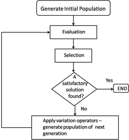
Evolutionary Computation (EC) or Evolutionary Algorithms (EA) is a class of optimisation algorithms based on an analogy with concepts of natural evolution. They belong to the more general class of machine learning algorithms, which are defined as [Mit96]: “computer algo-rithms that improve automatically through experience”. Algoalgo-rithms belonging to this class are mostly used as optimisation algorithms that seek to arrive at an optimal solution through the artificial simulation of evolution. Using a method to evaluate the quality of randomly generated solutions, the progress towards the optimum is achieved by mimicking survival of the fittest, and rewarding those deemed fitter by favouring them for reproduction.
Figure 2.4: Basic Evolutionary Algorithms Life Cycle
To design an EA, the following components must be in place:
• Representation: EA solutions are represented as collections of “genes”– called “somes”. The most basic form of representation is as a linear chromosome. The chromo-some is an encoding of the solution to the optimisation problem, and is also known as the
genotype.
2.2. Multiobjective Evolutionary Algorithms (MOEA) 17
• Quality indicator – Fitness function: designed to estimate how good a solution is in solving the given problem.
• Selection: the mechanism by which individuals from the population are selected to survive, and reproduce.
• Variation operations: as in nature, variation operations ensure exchange of genetic mate-rial between individuals (crossover), as well as the occasional changing of a random gene (mutation).
Different flavours of EAs exist, and each has been historically associated with a certain type of representation: Genetic Algorithms (GA): binary strings, Genetic Programming (GP): syntax trees, Evolutionary Strategies (ES): real-value vectors, and Evolutionary Programming (EP): finite state machines. However, these variations are mainly historical and varieties of representation within each EA exist. In the following section, we briefly introduce some background information on both GAs and GP. The life cycle of a typical EA algorithm is shown in Figure 2.4.
2.2.1.1 Genetic Algorithm
The GA was developed by John Holland in 1975 [Hol75]. The classic GA used a fixed length binary chromosome to encode solutions to the problem. Although the encoding of the solutions is problem specific and is up to the algorithm designer, the schemata theorem [Hol75, Gol89], which explains the mechanism by which the GA works, offers some guidelines on how to enhance the chromosome representation.
In the GA, the encoded chromosomes belong in the search space. To evaluate the fitness of the genotype, it is mapped onto the equivalent individual in the phenotypic space and is evaluated on the problem. Based on how well it solves the problems (achieves the objective), it is assigned a fitness value.
The variation operations used in the classic GA were crossover, mutation and sometimes copying of individuals as in the case when the reproduction operator or an elite survival mech-anism2is used. Crossover is typically used more heavily than the other operators, especially
mutation which is only used with a small probability. An example of the crossover operator is the one-point crossover, where a crossover point is chosen at random and the two parents exchange the part of the chromosome starting at the crossover point. Considering that the chromosome is a string of zeros and ones, the mutation operator simply flips the bit selected at random for mutation. Other varieties of both the crossover and mutation operators exist, especially as more complicated representations are being developed.
2.2.1.2 Genetic Programming
The term Genetic Programming was coined by Koza [Koz92] in which he suggested the use of a tree structure for the representation and automatic evolution of computer programs. He also
demonstrated in his seminal book, the wide variety of problems for which the algorithm can be used. Designing a GP algorithm requires specification of the following:
Figure 2.5: Sample Genetic Programming Tree Structure
• Representation: The GP uses a tree to represent its solutions (see Figure 2.5), the structure of the tree is not predefined, neither is its size, although sometimes a limit on the depth of the tree is imposed. GP trees consist of terminal and function nodes, where terminals provide input values to the system and function nodes process the input values and produce an output value. According to [BNKF98], the terminal setconsists of the inputs to the GP program, the constants supplied, and the zero argument functions. They are often calledleavesbecause they are located at the end of the tree branches. A leaf is a node that returns a numeric value, without itself having to take any input. [BNKF98] defines the function set asthe statements, operators, and functions available to the GP system. This set encompasses the boolean, arithmetic, trigonometric, logarithmic functions, conditional statements, assignment statements, loop statements, control transfer statement, et cetera. The focus of the encoding issue in the GP shifts from the design of the structure to the choice of the suitable terminal and function sets. Choosing a very large function and terminal sets complicates the search, while very small sets will be restrictive and may not allow for the evolution of appropriate solutions.
• Population: The population is initialised by generating random tree structures to fill the population. The trees are built from the terminal and function sets (except for the root node which can only be selected from the function set) such that the tree depth does not exceed the maximum allowed depth. There are three commonly used methods for building the trees. These aregrow, full, and ramped half-and-half [Hol75, BNKF98]:
1. The Grow method: In this method, nodes are selected randomly from the function and terminal set. Once a terminal node is added to a branch, this branch terminates whether or not the maximum depth has been reached. The tree structures in this method are often of irregular shape.
2.2. Multiobjective Evolutionary Algorithms (MOEA) 19
2. The Full method: Nodes are selected only from the function set until the node is at maximum depth, at which point they are selected from the terminal set. This method results in fully filled trees with all branches at the maximum depth.
3. The Ramped Half-and-Half method: Devised to enhance the diversity of the initial population. This method works as follows: Suppose the maximum allowed depth is 5, then the population is divided equally among individuals to be built with trees of depth: 2, 3, 4, and 5. For each depth group, half the trees are initialised with the full method and the other half are initialised with the grow method.
• Operators: There are many genetic operators that have been developed over the years. The three main GP operators are:
1. Crossover: The crossover operator swaps the genetic material of two parents in an attempt to propagate successful genetic material, and at the same time, vary the successful chromosomes so that the algorithm continues its exploration in the search space. One method for tree crossover would proceed by the following steps [BNKF98]:
– Select two parents based on the selection scheme used.
– Select a random subtree at each parent.
– Swap the selected subtrees. The resulting individuals are the children and are placed in the population of the next generation.
2. Mutation: Operates on one individual only. Many types of mutations exist. In one of them, a subtree is selected at random, removed from the individual and replaced by a randomly generated tree, following the same method for building a tree and adhering to the depth constraint.
3. Reproduction:The individual is copied and placed in the population.
• Fitness: The fitness function is a very important part of the GP as it is in all other evolutionary algorithms. It measures the success of an individual on the problem and in effect assigns its probability of reproducing and its genetic material surviving to the next generation. As the generations evolve, the average fitness of the population is expected to improve, which is a sign that the algorithm is learning.
• Selection:After the fitness of individuals has been determined, we need to decide which individuals will be allowed to propagate their genetic material, which will be kept in the population and which will be replaced. Some of the commonly used selection operators are [BNKF98]:
1. Fitness-Proportionate Selection: Employed in the classical generational GA, where the probability of an individual producing offspring is proportionate to the ratio of its
fitness to the average fitness of the population. This method is usually criticised for using an absolute measure for fitness.
2. Truncation Selection: Known in the ES community as (µ,λ), where a number of µ parents are allowed to produce λ offspring, out of which the best µ are used as parents in the next generation. This method is not dependent on the absolute fitness values, as theµbest will always be the best, regardless of the absolute fitness differences between individuals.
3. Ranking Selection: Individuals are sorted according to their fitness values, and given ranks. The selection probability is assigned as a function of their rank in the popu-lation.
4. Tournament Selection: Based on competition with a smaller subset of the candidate parents rather than the full population. A number of individuals, called the tourna-ment size, is selected randomly, then the best among those individuals is selected. The resulting offspring (or the mutated version of the individual) then replaces the worst individuals in the population. The tournament size plays a role in adjusting the selection pressure. A small tournament causes low pressure and a higher tour-nament sizes increase the selection pressure. The advantage of this method is that it gets rid of the centralised fitness comparisons among all individuals that have to be carried out in the other three methods, resulting in an acceleration of the selection process.
2.2.2 State of the Art Multiobjective Evolutionary Algorithms
Multi Objective Evolutionary Algorithms (MOEA) integrate the Pareto dominance concepts into the framework of the Evolutionary Algorithms (EAs). MOEAs are distinguished from standard EAs by employing the Pareto dominance concept in the fitness evaluation to allow for the comparison between individuals based on multiple conflicting objectives. Instead of producing one best solution, they produce a Pareto front of many solutions to the problem in one run. If the MOEA algorithm is successful, the solution set should be as close to the true Pareto front as possible, has a wide coverage of the front and be diverse enough to represent useful tradeoffs of the objectives [Coe05b].
MOEAs have received considerable attention in the last decade. They have been applied to a wide variety of application problems whose optimisation was characterised by the need for the simultaneous optimisation of conflicting objectives. The cycle of an MOEA, is the same as that of the EA, except when it comes to evaluating the fitness of individuals. In the following we present a review of some of the early MOEAs (MOGA,1993; NPGA, 1994; NSGA, 1994; PAES, 1999; and SPEA, 1999), as well as some of the more recent algorithms that were most prominently used in financial applications (PESA, 2000; NSGAII, 2001; and SPEAII, 2002). For a thorough review of these algorithms and others, the reader is referred to [Coe05a, TGC07].
2.2. Multiobjective Evolutionary Algorithms (MOEA) 21
Some of the most recent MOEA algorithms include: OMOPSO [RC05]; MOEA/D [ZL07, LZ09]; and SMPSO [NDG+09].
2.2.2.1 SPEA
This algorithm [ZT99] uses an elitism mechanism that employs an external archive for saving (preserving) the non-dominated solutions. The algorithm starts with a random population and an empty archive with a maximum predefined size. In each generation, all non dominated individuals are copied to the archive, which is then tested for dominated individuals, which are deleted if found. If the size of the archive exceeds the predefined limit, an agglomerative clustering technique based on phenotypic distance is used to delete some of the non-dominated individuals while preserving the diversity characteristics. Each member of the archive has a strength valueS(i)∈[0,1]. It is defined to be the number of the jpopulation members which are dominated by or equal to i, divided by the population size plus one. The Fitness F(j) of an individual j in the population is calculated by summing the strength valuesS(i) of all archive membersithat dominate or are equal toj, and adding one. In the reproduction phase, the current population and the archived population are mixed together to form one population from which parents are selected. Since the fitness values of the archive solutions are in the range of [0,1] and minimisation of fitness is sought, the archive members have more chance of being selected. The complexity of the algorithm was found to beO(mN2), wheremis the number of
objectives, andNis the size of the population. Although the algorithm is very successful in comparison with other algorithms, some weaknesses have been identified by Zitzler [ZLT02] as well as others. First, the fitness assignment in the population is based solely on the number of dominating individuals in the archive. This technique is not able to reflect information about dominance regarding members of the population itself, and the selection pressure can decrease significantly. Second, the clustering technique is used in the archive to maintain diversity; however, no technique is being used to maintain diversity in the population. Finally, in spite of the effectiveness of the clustering technique, it may lose outer solutions, even though they are still non dominating solutions that may be part of the Pareto front.
2.2.2.2 SPEA2
Designed by Zitzler, Laumanns and Thiele to overcome some weaknesses in the SPEA algorithm[ZLT02]. The SPEA2 algorithm also has an archive with a predefined size. The differences from SPEA are: (1) the archive in SPEA2 has a fixed size; if the number of non dom-inated individuals is less than the predefined size, the archive is filled with the best domdom-inated solutions from the population. On the other hand, if the archive is greater than the defined size, a truncation method is used instead of the clustering technique. (2) In the truncation method, individuals chosen for removal are those that have the minimum distance to another individ-ual. If several individuals have the same distance, the second smallest distance is considered. It was found that the truncation technique is better than clustering with respect to retaining the boundary points. (3) The fitness assignment in this algorithm is defined to take into account
both dominated and dominating solutions; each individual in both the archive and the popu-lation is assigned a strength value representing the number of solutions it dominates. On the basis of the strength value, the raw fitness value is calculated as the sum of the strengths of the individual dominators in both the archive and the population. Raw fitness is to be minimised; accordingly, non-dominated individuals will have a raw fitness value of 0. (4) In addition, density information is added to the fitness function by calculating the density as the inverse of the distance to thek-th nearest neighbour3. This is used as a mechanism to further discriminate
between individuals. The fitness of an individual is the sum of its raw fitness and density information. The complexity of the algorithm isO(M2) whereM=N+N0
, andN0is the archive size andNis the population size. (5) Only members of the archive participate in the mating selection process.
The SPEA2 was compared to SPEA as well as NSGAII. It was found that SPEA2 had a better distribution of points especially when the number of objectives increased, probably because of its maintenance of some dominated individuals which helped to maintain diversity.
2.2.2.3 NSGA
This algorithm was proposed in 1994 by Srinivas and Deb [SD94]. The population is ranked using Pareto dominance. The non-dominated individuals found are classified into one category and assigned a dummy fitness value proportional to the population size (the highest). This cat-egory is then excluded from the population, and another search for non-dominated individuals is conducted, until all of the population is ranked. To maintain diversity, individuals in each non-domination level are shared with their dummy fitness value.
Sharing fitness method: given a set ofnksolutions in thek-th non-dominated front, each
having a dummy fitness value fk, the sharing procedure is performed in the following way for
each solutioni=1,2, . . . ,nk:
• Step 1: Compute a normalised Euclidean distancedijmeasure with another solutionj. • Step 2: The distancedijis compared with a pre-specified parameterαshareand the following
sharing function value is computed as:
sh(dij)= 1− dij αshare 2 i f dij<αshare 0 otherwise (2.4)
• Step 3: Repeat for all j≤nk
• Step 4: Calculate niche count for thei-th solution as: mi=
Pnk
j=1sh(dij)
• Step 5: The shared fitness value fk0of thei-th solution is: fk0 = fk
mi, where fkis the solution’s
fitness value.
3Wherekis usually taken to be the square root of the sample size (population plus archive), and the distance is
2.2. Multiobjective Evolutionary Algorithms (MOEA) 23
Since individuals in each category obtain a fitness value proportional to their Pareto ranking ( with the first front getting the highest fitness value), their selection probability is proportional to the number of individuals they dominate. The algorithm is computationally expensive as it requires the comparison of each individual to every other individual in the population. In the worst case, where each front contains exactly one solution, the complexity of the algorithm is
O(mN3). The algorithm also requires the user to decide on the fitness sharing factor, for which
the performance of the algorithm has been shown to be very sensitive.
2.2.2.4 NSGAII
This algorithm was introduced by Deb et al. in 2001 [Deb01] as an improvement to the NSGA algorithm . They tried to overcome the main problem for which NSGA was criticised; its computational complexity. The new algorithm consists of two main loops. In the first, for each solutioni, two entities are computed: 1) The number of solutions which dominates it, denoted
ni, and 2) The number of solutions dominated by it, denotedSi. The calculation of these two
entities would requireO(mN2) comparisons. Next, the solutions withn
i=0 are identified and
are put in a separate listF1, which is called the current front. In the second loop, the current
front is traversed, and for every solution on it, each member jon itsSi list is visited and we
decrement its ownnj count by one. If the new decremented count becomes 0, it is put in a
separate listH. When all the members of the current front have been checked, the listF1 is
declared as the first front, andHbecomes the current front. The process is repeated withH
as the current front. Each iteration will requireO(N) computation. Since there are at mostN
fronts, then the worst case complexity of the second loop inO(N2) and the overall complexity
of the algorithm isO(N2)+O(N2)=O(N2). The fitness assignment, selection and reproduction
proceed as in the NSGA. The diversity is maintained by using a crowding measure in the selection and reproduction phase. The crowding measure is a density estimation technique in which for each solution, the density of solutions surrounding it is measured by the average distance of the two points on either side of that point along each of the objectives. This measure effectively calculates the largest cuboid enclosing a solution in the objective space without including any other solution.
2.2.2.5 MOGA
Fonseca and Fleming, 1993 [FF93b] presented a scheme in which each individual is given a rank proportional to the number of individuals in the population by which it is dominated. The non-dominated individuals are hence assigned the lowest rank of 1. The population is then sorted according to the rank. The fitness is assigned by interpolating from the best rank to the worst (Pareto ranking assignment). Then, the individuals with the same rank have their fitness averaged so they will be sampled at the same rate in the population. The algorithm requires a decision on a value for the fitness sharing factor.
2.2.2.6 NPGA
Proposed by Horn in [HNG94]. NPGA uses a tournament selection scheme based on Pareto dominance. However, instead of comparing two individuals to decide whether one of them dominates the other, the two individuals are compared to a random sample of the population. If one of them is non-dominated and the other is dominated with respect to the sample selected, then the non-dominated individual is returned. If both are dominated or non-dominated by the sample, then, the result of the tournament is decided through fitness sharing in the objective domain. The approach is faster than the previous ones, because it decides the Paret