Behavioral Dynamics on the Web: Learning, Modeling, and Prediction
Kira Radinsky, Technion—Israel Institute of TechnologyKrysta M. Svore, Microsoft Research Susan T. Dumais, Microsoft Research Milad Shokouhi, Microsoft Research Jaime Teevan, Microsoft Research Alex Bocharov, Microsoft Research Eric Horvitz, Microsoft Research
The queries people issue to a search engine and the results clicked following a query change over time. For example, after the earthquake in Japan in March 2011, the queryjapanspiked in popularity and people issu-ing the query were more likely to click government-related results than they would prior to the earthquake. We explore the modeling and prediction of such temporal patterns in Web search behavior. We develop a temporal modeling framework adapted from physics and signal processing and harness it to predict tem-poral patterns in search behavior using smoothing, trends, periodicities and surprises. Using current and past behavioral data, we develop a learning procedure that can be used to construct models of users’ Web search activities. We also develop a novel methodology that learns to select the best prediction model from a family of predictive models for a given query or a class of queries. Experimental results indicate that the predictive models significantly outperform baseline models that weight historical evidence the same for all queries. We present two applications where new methods introduced for the temporal modeling of user be-havior significantly improve upon the state of the art. Finally, we discuss opportunities for using models of temporal dynamics to enhance other areas of Web search and information retrieval.
Categories and Subject Descriptors: H.3.7 [Information Storage and Retrieval]: Digital Libraries; I.5.4 [Pattern Recognition]: Applications
General Terms: Algorithms, Experimentation
Additional Key Words and Phrases: Behavioral Analysis, Predictive Behavioral Models ACM Reference Format:
Radinsky, K., Svore, K., Dumais, S., Shokouhi, M., Teevan, J., Bocharov, A., and Horvitz, E. 2012. Behavioral Dynamics on the Web. ACM Trans. Inf. Syst. 0, 0, Article 0 ( 0), 37 pages.
DOI=10.1145/0000000.0000000 http://doi.acm.org/10.1145/0000000.0000000
1. INTRODUCTION
The way that people use Web search engines changes over time. We explore the tem-poral dynamics of Web search behavior, investigating how we can model and predict changes in queries that people issue, the informational goals corresponding to the queries, and the search results that they access during Web search sessions.
In information retrieval, models that incorporate user behavior signals typically ag-gregate evidence over time and use it identically for all types of queries [Agichtein
Author’s addresses: K. Radinsky, Computer Science Department, Technion—Israel Institute of Technology; Svore, K., Dumais, S., Teevan, J., Bocharov, A., and Horvitz, E., Microsoft Research, Redmond, WA; Shok-ouhi, M., Microsoft Research, Cambridge.
Permission to make digital or hard copies of part or all of this work for personal or classroom use is granted without fee provided that copies are not made or distributed for profit or commercial advantage and that copies show this notice on the first page or initial screen of a display along with the full citation. Copyrights for components of this work owned by others than ACM must be honored. Abstracting with credit is per-mitted. To copy otherwise, to republish, to post on servers, to redistribute to lists, or to use any component of this work in other works requires prior specific permission and/or a fee. Permissions may be requested from Publications Dept., ACM, Inc., 2 Penn Plaza, Suite 701, New York, NY 10121-0701 USA, fax+1 (212) 869-0481, or [email protected].
c
0 ACM 1046-8188/0/-ART0 $10.00
Japan query time series
Query time series: Japan
N o rm al iz e d # C li ck s (1 0 ^-6)
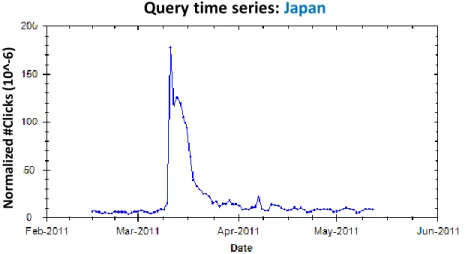
Fig. 1. A time series (2/14–5/25, 2011) for the queryjapan(normalized by overall #clicks logged on each day based on Bing query logs).
et al. 2006]. We learn to predict how the search behaviors of users change over time and use these predictive models to enhance retrieval. As an example, for a population of users, the frequency with which a query is issued and the number of times that search results are clicked for that query can change over time. In Figure 1, we show thetotal clicks1. We can see a dramatic change in behavior associated with this query
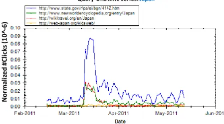
following the Japanese earthquake on March 11th, 2011. The number of clicks surges for the query for a period of time, and then slowly decays. Likewise, the URLs that people choose to click on following the same query may vary over time, indicating a change in what people consider as relevant for that query. Figure 2 shows the change in click frequency for several popular URLs following the queryjapanaround the time of the earthquake. The frequencies of access of some URLs (e.g., a US government site about Japan) mirror changes in query frequency, while others (e.g., a site for children to learn about Japan) do not change with query and click frequency.
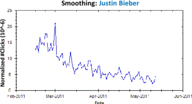
We model and predict these different kinds of search dynamics, focusing in particu-lar on predicting query and click frequency. Although the timing of the initial peak for the query japanmay be hard to predict, once it is reached, the subsequent behavior can be predicted. There are many other cases in which search behaviors are easy to predict. In Figure 3, the queryhalloweenexhibits periodic trends, andandroid under-goes an increasing trend in popularity, but the query justin bieberfluctuates with no obvious trend. Using time-series modeling, we can estimate these different trends and periodicities and predict future values of the frequency of queries and clicks. A major challenge is to select the appropriate model for predicting the dynamics. We present here a novel algorithm for selecting the best time-series model for each behavior, we re-fer to as thedynamics model learner(DML). Our model considers numerous factors for this selection, ranging from the long-term shape of the time-series to query-dependent features.
Learned models of what people search for, and then access via clicking on displayed results, can be used to improve the search experience. We shall consider two search-related applications: result ranking and query suggestion. When users information 1We definetotal clicksfor a queryqas the total number of times that any URL returned by the search engine in response to it is clicked.
Japan query-URL time series Query-URL time series: Japan
N o rm al iz e d # C li ck s (1 0 ^-6)
Fig. 2. Time series (2/14–5/25, 2011) for sample clicked URLs for queryJapan(normalized by total #clicks on each day based on Bing query logs).
Fig. 3. Different classes of temporal trends in query frequencies.
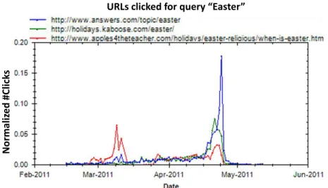
needs change over time, the ranking of results should also change to accommodate these needs. Consider the example presented in Figure 4, which shows the frequency of URL clicks for the queryeasterat different times during the year. A user’s informa-tion need several weeks before the Easter holiday (in mid-March) is likely to identify the exact date of the holiday; indeed, the URL when-is-easter.html is clicked more often than other Easter-related pages during mid-March. A few days before Easter, people issuing this query appear to become more interested in planning activities for the holiday, and logs of clickthroughs show that sites such asholidays.kaboose.comare clicked more often than other pages during this period of time. During Easter itself, people seem to be more interested in the religious meaning and customs of the holiday, questions that are answered by pages such asanswers.com/topic/easter. To account for changes in what people click on following a query likeeaster, we explore time-aware ranking mechanisms using two ranking scenarios. The first predicts user click behav-ior for a given day using only this prediction to rank URLs. The second approach uses temporal user behaviors as features (along with content-based features) in a learning-to-rank algorithm. We find that weighting user behavior for each query and URL pair based on temporal dynamics significantly improves the accuracy of the ranked results in both types of ranking scenarios across several types of queries.
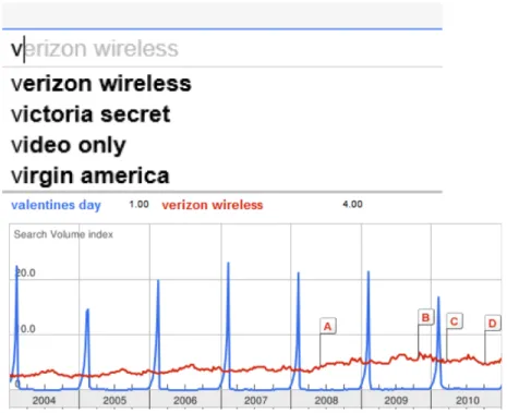
We also explore the application of our methods for time-aware query auto-suggestion (QAS), also calledauto completion. Consider the example presented in Figure 5. On February 13th 2012—a day before Valentine’s day— Google suggestedverizon wire-less as a top candidate forv(underlined) and did not suggest any Valentine-related
URLs clicked for query “Easter” No rma liz ed #C lick s
Fig. 4. Clicked-URLs behavior (2/14–5/25, 2011) for the queryeaster (normalized by the total #clicks on each day and the position of the URL).
candidates in the QAS ranking (the top plot in Figure 5).2The query frequency trends
in the bottom plot of Figure 5 however clearly show thatvalentines dayis a more rele-vant suggestion during this time period. We use the same time-series models to predict the query frequency and demonstrate that modeling the temporal profile of queries can improve the ranking of auto-suggestion candidates.
In summary, the key contributions described in this paper are as follows:
— We highlight the rich opportunities to study the dynamics of Web search behavior and explore several time-series models to represent and predict different aspects of search behavior over time. We discuss how these models can be learned from histori-cal user-behavior data, and develop algorithms tailored to address several aspects of the dynamics of population behavior on the Web, includingtrend, periodicity, noise, andsurprise.
— We present a new learning algorithm, which we refer to as the dynamics model learner(DML), that determines the appropriate model to use for predicting behavior, based on features extracted from large-scale logs of Web search behavior over time. We show that DML performs better than more traditional model selection techniques. — We perform empirical evaluation of our approaches over large-scale logs of real-world user behavior (obtained from Bing), providing evidence for the value of temporal modeling techniques for capturing the dynamics observed in populations of users on the Web.
— We present applications of our temporal modeling methods to improve ranking and query suggestions, and provide evidence for the superiority of temporal modeling in both applications.
2. RELATED WORK
Several lines of research are related to modeling and predicting peoples’ Web search behavior over time [Lau and Horvitz 1998]. We begin our discussion of related work with a review of studies that have characterized temporal search behavior dynamics 2The query was issued from the United States with personalization disabled.
Fig. 5. (Top) The auto-suggestion candidates ranked by Google on the 13th of February 2012, a day before Valentine’s Day in the USA. (Bottom) Query frequencies forvalentines dayvs.verizon wirelesssince 2004.
on the Web. We next summarize previous research that has used temporal evidence for ranking, mostly focusing on content dynamics rather than behavioral dynamics. Finally, we describe related work in automatic query suggestion.
2.1. Web Search Behavioral Dynamics
The variations of query volume over time have been studied extensively in prior work. For example, some researchers have examined changes in query popularity over time [Wang et al. 2003] and the uniqueness of topics at different times of the day [Beitzel et al. 2004]. Some studies [Jones and Diaz 2007] identified three general types of tem-poral query profiles: atemtem-poral (no periodicities), temtem-porally unambiguous (contain a single spike), and temporally ambiguous (contain more than one spike). They fur-ther showed that query profiles were related to search performance, with atemporal queries being associated with lower average precision. Kulkarni et al. [2011] explored how queries, their associated documents, and the intents corresponding to the queries change over time. The authors identify several features by which changes in query popularity can be classified, and show that presence of these features, when accom-panied by changes in result content, can be a good indicator of change in the intent behind queries. Others [Chien and Immorlica 2005; Radinsky et al. 2011; Wang et al. 2007] used temporal patterns of queries to identify similar queries or words.
Vlachos et al. [2004] were among the first to examine and model periodicities and bursts in Web queries using methods from Fourier analysis. They also developed a method to discover important periods and to identify query bursts. Shokouhi [2011] identified seasonal queries using time-series analysis.
Shimshoni et al. [2009] studied the predictability of search trends using time-series analysis. Kleinberg et al. [Kleinberg 2002; 2006] developed general techniques for sum-marizing the temporal dynamics of textual content and for identifying bursts of terms within content.
Researchers have also examined the relationship between query behavior and events. Radinsky et al. [2008] showed that queries reflect real-world news events, and Ginsberg et al. [2009] used queries for predicting H1N1 influenza outbreaks. Similarly, Adar et al. [2007] identified when changes in query frequencies lead or lag behind men-tions in both traditional media and blogs. From a Web search perspective, breaking news events are a particularly interesting type of evolving content. Diaz [2009] and Dong et al. [2010b] developed algorithms for identifying queries that are related to breaking news and for blending relevant news results into core search results. K¨onig et al. [2009] studied click prediction for news queries by analyzing the frequency and location of keywords in a corpus of news articles. Information about time-varying user behavior was also explored by Koren [2009], who used matrix factorization to model user biases, item biases, and user preferences over time.
Although much has been done to understand user Web search behavior over time, few efforts have sought to construct underlying models of this behavior and then used these models to predict future behavior. We present the construction of models for behaviors over time that can explain observed changes in the frequency of queries, clicked URLs, and clicked query-URL pairs.
2.2. Using Temporal Dynamics for Ranking
Agichtein et al. [2006] were the first to show that user behavior data could significantly improve ranking. In that work, the user behavior was represented as the simple aver-age of behaviors over time, independent of query, URL clicks, or interactions between the two.
Researchers have examined how temporal attributes can be used to improve rank-ing usrank-ing various kinds of content analysis. Dakka et al. [2008] defined a class of time-sensitive news queries, and suggested an approach that identifies important time in-tervals for those queries and augments the weight of those documents for ranking. Metzler et al. [2009] investigated a subset of temporal “year queries” – i.e., queries that often include the addition of terms representing a year such asSIGIR 2012, and modified the language model of the document so that that years found in the docu-ment are weighted more heavily. Similarly, Efron and Golovchinksy [2011] and Li and Croft [2003] added temporal factors into models of language likelihood and relevance for re-ranking results based on the publication date of documents. Elsas and Dumais [2010] incorporated the dynamics of content changes into document language models to improve relevance ranking, showing that there is a strong relationship between the amount of change and term longevity and document relevance. Efron [2010] considered term popularity in a document collection over time, to adjust term weights for docu-ment ranking. In summary, the prior studies cited above examine how general changes in content or specific content features (like dates) can be used to improve ranking.
Another line of research centers on methods for improving the ability of search en-gines to rank recent information effectively. Diaz [2009] studied how news can be inte-grated into search results by examining changes in query frequency, the popularity of query terms in the news collection, and query click feedback on presented news arti-cles. Dong et al. [2010b] used Twitter data to detect and rank fresh documents. Simi-larly, Dong et al. [2010a] identified queries that are time-sensitive, developed features that represent the time of Web pages, and learned a recency-sensitive ranker. Dai et al. [2011] presented a ranking optimization with temporal features in documents, such as the trend and seasonality of the content changes in title, body, heading, anchor, and
page or link activities. In summary, this line of research focuses on the desirability of providing fresh results for some kinds of queries.
To the best of our knowledge, temporal characteristics of queries and clickthrough behavior have not yet been used to improve general ranking of documents. In this work, we use time-series models to represent the dynamics of search behavior over time and show how this can be used to improve ranking and query suggestions. 2.3. Query Auto-Suggestion
In addition to using temporal models for ranking, we also use them to improve query auto-suggestion (QAS). Previous work on query auto-suggestion can be grouped into two main categories. The first group (also referred to as predictive auto-completion [Chaudhuri and Kaushik 2009]) uses information retrieval and NLP techniques to generate and rank candidates on-the-fly as the user enters new words and charac-ters [Darragh et al. 1990; Grabski and Scheffer 2004; Nandi and Jagadish 2007]. For instance, Grabski and Scheffer [2004], and Bickel et al. [2005] studied sentence com-pletion based on lexicon statistics of text collections. Fan et al. [2010] ranked auto-suggestion candidates according to a generative model learned by Latent Dirichlet Allocation (LDA) [Blei et al. 2003]. White and Marchionini [2007] developed a real-time query expansion system that produces an updated list of candidates based on the top-ranked documents as the user types new words in the search box.
In the second group of QAS techniques — including the one presented here — can-didates are pre-generated and stored in tries and hash tables for efficientlookup. The list of candidate suggestions is updated by new lookups with each new input from the user. The filtering of candidates is typically based on exact prefix matching. Recently, Chaudhuri and Kaushik [2009] and Ji et al. [2009] proposed flexible fuzzy matching models that are tolerant to small edit-distance differences between the query (prefix) and candidates.
In the context of Web search, the most conventional approach is to rank candidate query suggestions according to their past popularity. Bar-Yossef and Kraus [2011] re-ferred to this approach asMostPopularCompletion(MPC):
MPC(P) = arg max q∈C(P)w(q), w(q) = f(q) P i∈Qf(i) . (1)
where, f(q)denotes the number of times the queryq occurs in a previous search log Q. They propose a context-aware technique in which the default static scores for the candidates are combined with contextual scores based on recent session history to compute the final ranking. Under the MPC model, the candidate scores do not change as long as the same query log Q is used. We also take MPC [Bar-Yossef and Kraus 2011] as our QAS ranking baseline and show that it can be improved significantly by considering the temporal characteristics of queries.
Our approach is distinct from prior work in several important ways. We use time-series analysis to learn how to differentially weight historical click data for queries, URLs, and query-URL pairs (extending the work by Radinsky et al. [2012]). This en-ables recent behavior to be weighted more highly for some queries (or URLs or query-URL pairs) but not others; and similarly for periodic behaviors to be important for some queries but not others; etc. Second, we extend previous research on ranking fresh results by addressing the more general challenge of finding the most appropriate re-sults, even if they are not recent. We extend earlier work by Agichtein et al. [2006] on search ranking by harnessing time-series analyses to learn the most appropriate weighting of previous behaviors rather than simply averaging previous behavior. Fi-nally, we show that the temporal profiles of queries created by our time-series models
can be used to improve the ranking of query auto-suggestion candidates that have his-torically been based on static measures of popularity (extending the early results by Shokouhi and Radinsky [2012] with further experiments and insights).
3. TEMPORAL MODELING OF WEB SEARCH BEHAVIOR
We now present a modeling technique based on state-space models that we use to capture the dynamics of Web behavior. Of special importance in modeling Web search behavior are global and local trends, periodicities, and surprises. We summarize in this section a general theory behind this model and discuss several modeling techniques we use to capture these important aspects. We conclude the section with a discussion of how the models can be used.
3.1. Model Framework: State-Space Models
The state-space model (SSM) is a mathematical formulation frequently used in work on systems control [Durbin and Koopman 2008] to represent a physical system as a set of input, output, and state variables related by first-order differential equations. It provides an easy and compact approach for analyzing systems with multiple inputs and outputs. The model mimics the optimal control flow of a dynamic system, using some knowledge about its state variables. These models allow for great flexibility in the specification of the parameters and the structure of the problem, based on some knowledge of the problem domain that provides information about the relations (e.g., linear) among the parameters. We use upper-case letters for matrices and lower-case for scalars. The linear space state model (with additive single-source error) defines a system behavior by the following two equations:
Yt=W(θ)Xt+t, (2)
X(t+1)=F(θ)Xt+G(θ)t, (3)
where Yt is the observation at timet, Xt is the state vector,t is a noise series, and
W(θ), F(θ), G(θ)are matrices of parameters of the model. For a longer prediction range
h (also referred to as the prediction horizon), it is usually assumed that Yt+h = Yt. For simplicity, in the following sections we present equations for h= 1. We shall as-sume (as commonly asas-sumed in representations of dynamics in natural systems) that
tare independent and identically distributed following a Gaussian distribution with varianceσ2 and mean0. Equations (2) and (3) are called the measurement and
tran-sition equations, respectively. To build a specific SSM, a structure for the matrices
W(θ), F(θ), G(θ)is selected, and the optimal parametersθandσ and an initial state
X0are estimated.
The SSM representation encompasses all linear time-series models used in practice. We show in this section how the SSM can be applied to model query and click frequency in Web search. We model the stateXtusing a trend component and a seasonal (or pe-riodicity) component, as is often done for modeling time series [Hyndman et al. 2008]. The trend represents the long-term direction of the time series. The seasonal compo-nent is a pattern that repeats with a known periodicity, such as every week or every year. We first present models for user search behavior using just historical smoothing, and then present models with trend, periodicity, and their combination. Finally, we explore models that incorporate notions of unexpected observations orsurprises. Each model is represented by setting the scalars of the matricesW(θ), F(θ), G(θ).
Smoothing: Justin Bieber N o rm al iz e d # C li ck s (1 0 ^-6)
Fig. 6. Query exhibiting behavior where historical data has little relevance for predicting future clicks (normalized by overall #clicks on each day based on Bing query logs).
3.2. Modeling with Smoothing (SMT)
For the queryjustin bieberin Figure 6, simple averaging of past frequencies may give too much weight to the relatively high popularity of the query before April, and hence if used for forecasting, it is likely to overestimate the future popularity.
Therefore models that simply average historical data, and then extrapolate a con-stant value as a prediction, may perform poorly for predicting the future. The simple moving average technique, also called the simplest Holt-Winters model [Holt 2004], is a technique for producing an exponentially decaying average of all past examples, thus giving higher weights to more recent events. The model is represented by the following equation,
yt+1=α·xt+ (1−α)·yt. Here, fory=x0, solving the recursive equation as follows,
yt+1=αxt+. . .+α(1−α)k−1xt−k+. . .+ (1−α)tx0
produces a predictionyt+1 that weights historical data based on exponentially decay
according to the time distance in the past. The parameterαis estimated from the data (see Section 3.7). Converting to SSM notation, letlt=yt+1whereltis the level of the time series at timetandt=xt−yt. The measurement and transition equations can be defined as:
Yt=yt=lt−1, (4)
Xt=lt=lt−1+αt. In this case,W = (1), F = (1), G= (α).
3.3. Modeling Trends (TRN)
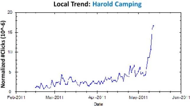
In many cases, such as the queryharold campingin Figure 7, using only one coefficient to discount previous data does not have the expressiveness to capture the dynamics of the system. The figure shows the query-click behavior for the queryharold camping, who predicted that the end of the world would commence on May 21st, 2011. The growing interest in this prediction in the proximity of this date shows a clear local growth trend in the time series. In such cases, where the time series exhibits a local trend, simple smoothing of historical data cannot accurately capture the dynamics of
Local Trend: Harold Camping N o rm al iz e d # C li ck s (1 0 ^-6)
Fig. 7. Query exhibiting behavior with local trend (normalized by overall #clicks on each day based on Bing query logs).
interest in the topic. A potential solution to this problem is the addition of a trend componentbtto the previously described model:
yt=lt−1+d·bt−1+t, (5)
lt=lt−1+bt−1+αt,
bt=bt−1+β∗(lt−lt−1−bt−1),
whereltis called the level of the time series at timet,dis thedamping factor, andbt is theestimation of the growth of the seriesat timet, which also can be written as
bt=bt−1+αβ∗t=bt−1+βt. LetXt= (lt, bt)0, then: Yt= (1 d)Xt−1+t, Xt= 1 1 0 1 Xt−1+ α β t. In this case,W = (1 d), F = 1 1 0 1 , G= α β .
The parametersα, βare estimated from the data (see Section 3.7). 3.4. Modeling Periodicity (PRD)
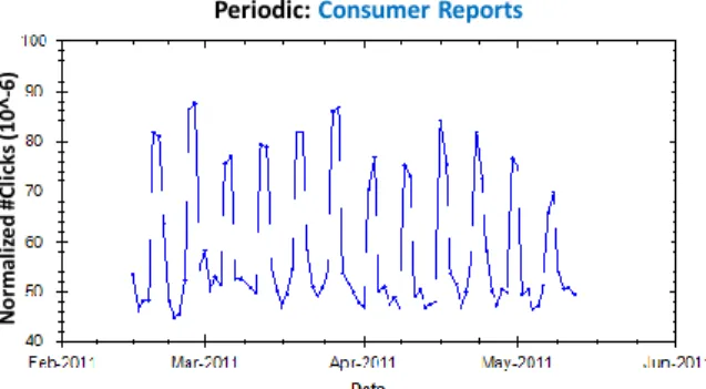
Figure 8 shows query-click behavior for the queryconsumer reportthat exhibits weekly periodicity. Similarly, the queryhalloweenin Figure 3 exhibits annual periodicity. For such queries, predictions based only on local trends or smoothing of the data will per-form badly during the peaks. A possible solution is the addition of a periodic or sea-sonal componentstto the simple Holt-Winters model,
yt=lt−1+st−m+t,
lt=lt−1+αt,
st=γ∗·(yt−lt−1) + (1−γ∗)st−m,
where mis the periodicity parameter that is estimated based on the data along with other parameters (see Section A.1 for details). In SSM notation, the equation system can be written as:
Periodic: Consumer Reports N o rm al iz e d # C li ck s (1 0 ^-6)
Fig. 8. Query exhibiting a periodic behavior (normalized by overall #clicks on each day based on Bing query logs).
yt=lt−1+st−m+t, (6)
lt=lt−1+αt,
st−i=st−i+1,
. . . , st=st−m+γt,
and forXt= (lt, s1, . . . , sm), we can represent the parametersF, G, W in a form of the matrices similar to the Trend Holt-Winters model formulation. The parameters α, γ
are estimated from the data (see Section 3.7). 3.5. Modeling Trends and Periodicity (TRN+PRD)
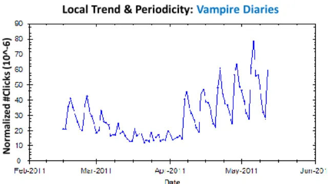
In the previous models, trend and periodicity were considered separately. However, for many queries, such as the query vampire diaries shown in Figure 9, the trend and periodicity components are mixed. In this case, the periodicity is unchanged but the frequency increases. The addition of trend and periodicity parameters produces the following model: yt=lt−1+d·bt−1+st−m+t, (7) lt=lt−1+bt−1+αt, bt=bt−1+βt, st=st−m+γt, . . . , st−i=st−i+1.
The parametersα, β, γare estimated from the data (see Section 3.7). 3.6. Modeling Surprises (SRP)
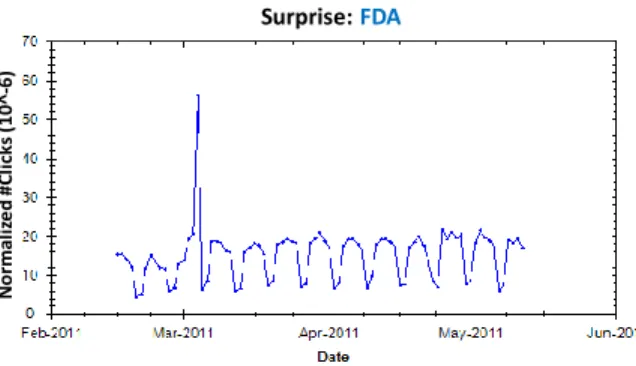
The Holt-Winters models assume the conversion of a set of parameters to a single fore-cast variable Yt. However, in many real-world time series, the model itself changes over time and is affected by external disturbances caused by unmodeled, exogenous processes in the open world. For example, in Figure 10, we see a periodic queryfda with a disturbance on March 4th, due to an external event concerning the announce-ment that some prescription cold products are unsafe. Inclusion of such outliers might
Local Trend & Periodicity: Vampire Diaries N o rm al iz e d # C li ck s (1 0 ^-6)
Fig. 9. Query exhibiting periodic behavior with local trend (normalized by overall #clicks on each day).
have a strong effect on the forecast and parameter estimation of a model. We wish to identify characteristics in the temporal patterns which are not adequately explained by the fitted model, and try to model them for a better estimation ofYt. If these charac-teristics take the form of sudden or unexpected movements in the series, we can model them by the addition of disturbancesthat capture the occurrences of surprises from the perspective of the model.
A disturbance or asurprise is an event which takes place at a particular point in the series, defined by its location and magnitude. In a time series, the effect of a dis-turbance is not limited to the point at which it occurs, but also propagates and creates subsequent effects that manifest themselves in subsequent observations.
We augment the standard Holt-Winters model with the addition of twosurprise pa-rameters:mt, which is a surprise measurement at timet, andkt, which is the surprise trend at timet: yt=lt−1+d·bt−1+st−m+mt+t, (8) lt=lt−1+d·bt−1+αt, bt=bt−1+kt+βt, st=st−m+γt, . . . , st−i=st−i+1.
We discuss in Section A.2 methods for identifying the surprisesktin a time series, and in Section 3.7 discuss how the parametersα, β, γare estimated from the data.
3.7. Using the Models to Forecast
Once the model structure is specified, the distribution of the future values of the time series can be evaluated, given past history. That is, we learn an SSM for time series
Y1, . . . , Yn jointly with the internal statesX0, . . . , Xn, and residuals0, . . . , n. During prediction, future states Xn+1 are generated using the state transition equation (Eq.
3) and, based on these, a distribution of the future values Yn+1 is generated using
the measurement equation (Eq. 2). The final prediction can be generated by using the expected value of this distribution.
The SSM family provides a predefined structure for forecasting, where the specific parameters of the model need to be evaluated from the data. We apply gradient descent [Snyman 2005] to optimize the model parameters based on training data. We assume here the following loss function, which is a common criterion for measuring forecast
Surprise: FDA N o rm al iz e d # C li ck s (1 0 ^-6)
Fig. 10. Query exhibiting behavior with surprises.
error: F = T X t=1 2t. (9)
The initial values of the models,X0, are set heuristically, and refined along with the
other parameters. The seasonal componentmis estimated from the data by autocorre-lationanalysis (see Section A.1 for details).
4. LEARNING THE RIGHT TEMPORAL MODEL
As described in Section 3, different temporal models can be employed to represent user behaviors over time. We first present a known method for selecting which model is the best based on the information criterion of the time series (Section 4.1), and then provide a novel method for inferring the model based on extended and domain-specific characteristics of Web behaviors (Section 4.2).
4.1. Bayesian Information Criterion
The models described thus far are based on curve fitting and we have shown via ex-amples that there is no single model that adequately models trends, periodicities, and surprise. An alternative approach would be tofitseveral models, and train a classifier that selects the best predictive model.
Each model adds more parameters. When fitting the models, there is a high likeli-hood of more complex models fitting the data better. This might result in overfitting, especially when applying gradient descent. The Bayesian information criterion (BIC) [Schwarz 1978] resolves this problem by adding a penalty for the number of parame-ters in the model. That is, it presents a tradeoff between the accuracy and the complex-ity of the model. It is closely related to the Akaike information criterion (AIC), but the penalty term is larger in BIC than in AIC. The BIC criteria being optimized is defined as:
BIC =−2·log(L) +q·log(n), (10)
where qis the number of parameters,nis the length of the time series, andLis the maximized likelihood function. For a Gaussian likelihood, this can be expressed as
whereσeis the variance of the residual in the testing period (estimated from the test data). The model with the lowest BIC is selected to represent the time series and to issue point forecasts.
4.2. Dynamics Model Learner (DML)
The BIC criterion introduced in Section 4.1 takes only the model behavior on the time-series values into account. However, in our domain we have access to richer knowledge about search behavior. For example, we know what query was issued, the number of clicks on a given URL for that query, and so on. We shall now discuss how to use domain knowledge to further improve behavior prediction. We focus on learning which of the trained temporal SSM models is most appropriate for each object of interest, and then estimating parameters for the chosen model.
4.2.1. Going Beyond Time-series for Temporal Modeling.We start by formally motivating the algorithm and defining the learning problem. LetT be the discrete representation of time andObe the set of objects, and letfi:O×T →F(fi)be a set of features. For example,Ocan be a set of URLs,f1(o, t)can be the number of times URLowas clicked
at timet, andf2(o, t)can be the dwell time on the URL at timet.
In time-series analysis, asingle object ois modeled over some periodt1, . . . , tn, and
a model C : T → R can be trained based on those historical examples. In order to
forecast future trends (classes) at timeti+1, the model is provided with an example of
the object seen at training timeti(for example, predicting how many times the URLo is clicked on tomorrow based on its past history).
In regression learning, multiple objects O0 ⊂ O are modeled simultaneously by a single model C : O → R. During prediction, the regression model may be given an
example of an objectoi, that has not been seen before, to produce the prediction of its numeric value. Notice that no notation of time is considered.
The time-series approach is capable of making specific predictions about a specific object at a certain time, but does not consider information about other objects in the system and therefore cannot generalize based on their joint behaviors. Regression learning, on the other hand, generalizes over multiple objects, but does not use the specific information about the object it receives during prediction, and therefore does not usually use the information about how this specific object behaves over time.
We combine the two approaches into a unified methodology that first considers gen-eralized information about other objects to choose a model of prediction and then uses the specific knowledge of the predicted object to learn the specific parameters of the model for the object. Formally, given a set of objectsO0 ⊂O over some period of time
t0, . . . , tn, we produce a modelCthat receives an objecto∈O(not necessarilyo∈O0)
over some period t0, . . . , tn, and produces the prediction of its numeric value at time
tn+1.
4.2.2. DML Learning. In this section, we present thedynamics model learner (DML) algorithm for learning from multiple objects with historical data. LetO0 ⊂Obe a set of objects given as examples for training the learning model. Lett1, . . . , tn+σbe the times dedicated for training the model. For example, O0 can be a set of queries for which we have user behavior information for the period of time t1, . . . , tn+σ. We divide the
objects into two sets — the learning set,t1, . . . , tn, and the validation settn+1, . . . , tn+σ.
For every temporal model described in Section 3, we train a model on the learning period, and check the mean squared error (MSE) over the validation period. Formally, let o(t) be the behavior of objecto at time t (e.g., how many times the query o was
searched), then M SE(o, t1, . . . , tn+σ, m) = Ptn+σ t=tn+1(o(t)−bo(t)) 2 σ ,
wherebo(t)is the modelmestimation at timet.
Letibe the index of the model with the lowest MSE on the test period for the object
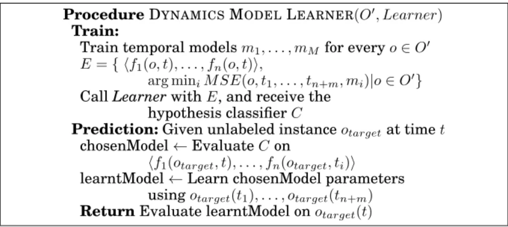
o. We construct a set of examplesE ={hf1(o, t), . . . , fn(o, t)i, i|o∈ O0}— a vector rep-resenting an object and labeled with the index of the best-performing model for that object. We then use a learner (in our experiments, a decision-tree learner) along with the examplesEto produce a classifierC. During prediction,Cis applied on the object we wish to predict,otarget. The outputm=C(otarget)represents the index of the most appropriate model for the object otarget. We train the modelm using the behavior of
otarget duringt1, . . . , tn+σ. A detailed algorithm is illustrated in Figure 11. An exam-ple of a learned decision tree is shown in Figure 12. In this figure, we see that the periodic model should be applied only on objects (queries) considered periodic (as de-fined in Section A.1), along with other characteristics. If the query is not periodic, the trend or the smoothing model should be applied, depending on the query shape (see Section 4.2.3). Thus, by using the DML model we learn to apply the best equations for modeling the time series.
ProcedureDYNAMICSMODELLEARNER(O0, Learner)
Train:
Train temporal modelsm1, . . . , mM for everyo∈O0
E={ hf1(o, t), . . . , fn(o, t)i,
arg miniM SE(o, t1, . . . , tn+m, mi)|o∈O0}
CallLearnerwithE, and receive the hypothesis classifierC
Prediction:Given unlabeled instanceotargetat timet
chosenModel←EvaluateCon
hf1(otarget, t), . . . , fn(otarget, ti)i learntModel←Learn chosenModel parameters
usingotarget(t1), . . . , otarget(tn+m)
ReturnEvaluate learntModel onotarget(t)
Fig. 11. The procedure estimates the model type to learn based on past examples and their features. The model parameters are estimated and a prediction for the new object is performed.
4.2.3. DML Features. DML uses a set of featuresfiabout each objecto. In this section, we discuss the specific features we use to train the DML model used in our experi-ments. We devise a total of 973 features (description of the features is available online
3), and group them into three groups: aggregate features of the time series o, shape
features of the time series o, and other domain-specific features such as the query class.
Aggregate Features. Features include theaverage,minimum,maximum, andperiod of the time series, e.g., the average of the query volume. Other features consider the dynamics of the series, e.g., the time seriesperiodicityandnumber of surprises. We also consider thesize of the spikesduring the surprises (the magnitude of the disturbance). 3
Is Query Periodic? urlImpression_quefrancy1 <= 29.66 queryurlAVG <= 0.04 urlImpression quefrancy10 <= 13.72 Query Period <= 130
URL Peaks AVG<= 0 Query Period <= 126: Smoothing (Eq. 3) Query Period > 126: Periodic (Eq. 5) queryurlImpression_LastValue <= 6 urlImpression_quefrancy_3 <= 5.12 urlImpression quefrancy5 <= 5.76:
Local Trend (Eq. 4)
urlImpression quefrancy_5 > 5.76:
Smoothing (Eq. 3)
NO YES
Fig. 12. A part of the learned dynamic model.
Shape Features. Shape features represent the shape of the time series. Our goal is to produce a representation that is not sensitive to shifts in time or to the magnitude of the differences. Formally, for a time seriesy[n] =x[n], we are looking for a represen-tation that will be equivalent to series of the formy[n] =x[n−h]andy[n] =A·x[n], for any shifthand any scalarA. Homomorphic signal processing is a solution that sat-isfies these conditions. Intuitively, application of the Finite Fourier transform (FFT) operator on a time series transforms it to what is called thespectral domain, i.e., pro-duces a vector xof size k, where every xk represents the k-thfrequency of the time series. xk = N−1 X n=0 xne−i2πk n N
This procedure eliminate shifts, as bothy[n] =x[n−h]andy[n] =x[n]have similar frequencies. Application of a log function on the resulting frequency vector and an additional FFT operator transforms it to what is called thecepstral domain[Childers et al. 1977], and the values of xin this product are calledquefrencies. The byproduct of these procedures is that series of the form y[n] = A·x[n−h] and y[n] = x[n] are transformed to the same vectorX in the ceptral domain. In speech recognition [Bogert et al. 1967], the values of x1, . . . , x13 in the cepstral domain are considered a good
representation of the series. We consider these features to represent the shape of the series.
Domain-Specific Features. We also consider a set of temporal and static features that are domain specific. For the query-click time series we consider the totalnumber of clicked URLs, and thequery-click entropyat timet, which is defined as:
QueryClickEntropy(q, t) =− n X
i=1
p(clickt(ui, q)) logp(clickt(ui, q)), (12) where u1, . . . , un are the clicked URLs at time t, and p(clickt(ui, q))is the percentage of clicks on URL ui for query q at time t, among all clicks on query q. If all users click on the same URL for query q, then QueryClickEntropy(q, t) = 0. We consider an aggregated version of query-click entropy as the average of the last k = 7days
before the prediction. For both the query and URL click time series, we consider the topical distributionof the URL or query. We used a standard topical classifier which classifies queries into topics based on categories from the Open Directory Project (ODP) [Bennett et al. 2010]. We classify queries into approximately 40 overlapping topics, such as travel, health, and so on.
5. OVERVIEW OF APPLICATIONS OF TIME-SERIES MODELING FOR SEARCH
Models that take advantage of historical user behavior data often aggregate the data uniformly, regardless of when the behavior is observed. These techniques fail to weight older data differently than newer data and may lead to a stale user experience. We now explore how the time-series modeling techniques presented in previous sections can be applied to resolve this problem. We first summarize how we predict future clicks and then describe two important search-related applications: ranking and query auto-suggestion. In Sections 6, 7, and 8 we provide the experimental results of those applications.
5.1. Experiments for Predicting Future Clicks
We start with an application of the methods we described for click prediction, and investigate three types of forecast: query click prediction, query-dependent URL click prediction, and query-independent URL click predictions. We extend the early results presented in Radinsky et al. [2012]. We provide a deep analyze the performance of different temporal models on the different types of predictions and their behavior for different prediction horizons (Section 6).
5.2. Experiments for Ranking Search Results
Web search engines often rely on usage data such as clicks and anchor text for rank-ing documents. Such techniques tend to favor older documents that have accumulated more behavioral data over time over fresher and potentially more relevant documents. As an example (shown in Figure 13), one of the highest ranked results for the query WSDM conferenceat the time of writing this paper is the WSDM 2010 (on Bing) or WSDM 2011 page (on Google). However, the current intention behind this query is more likely about finding information on the forthcoming WSDM 2013 conference. The older pages have more historical data than the more recent one, which only has sparse click data because it did not even exist prior to 2012. Accurate predictions of future query and click frequency can be used directly to ranking the search results. We re-fer to those predictions astemporal features. Alternatively, those features can be used along with other features to train a ranking function, e.g., BM25 features [Robertson et al. 2004]. We refer to those features asbase features.
We explore both of these scenarios. In our first set of ranking experiments, we lever-age temporal features as independent evidence for ranking. To understand how well our predictions can be used as independent evidence for ranking, we only use our pre-diction of future user behavior. For each query-URL pair we compute the predicted normalized number of clicks and use that prediction to rank the URLs.
In the second set of ranking experiments, we use temporal features as input to a learning-to-rank algorithm. We employ a supervised learning technique to learn the ranking function that best predicts the ground-truth ranking of URLs for a given query, using a variety of query, query-URL and URL features, combining both base features and temporal features. We show that rankers that use temporal modeling consistently outperform rankers only considering static user behavior.
We provide an analysis of the temporal models applied to ranking search results in Section 7.
Fig. 13. Search results for the queryWSDM conferenceon August 5th 2012. The 2010 (left im-age) and 2011 (right imim-age) conference websites are ranked higher than the 2013 conference website.
5.3. Experiments for Ranking Query Auto-Complete Candidates
Query auto-suggestion (QAS) is a feature incorporated in most search engines, where the goal is to save user time by predicting user’s intent and suggesting other possible queries matching the first few keystrokes typed. In a typical QAS scenario, the user is presented with a list of query suggestions that match the prefix text entered in the search box so far (e.g., “di” in Figure 14). For each prefixP, the list of candidatesC(P) consists of all previous queries that start withP4. The list of candidates is dynamically
updated at run-time with each new character typed by the user.
The common practice for ranking QAS candidates is to use past query frequencies [Bar-Yossef and Kraus 2011; Chaudhuri and Kaushik 2009] aggregation as a proxy for theexpectedpopularity in the future. Bar-Yossef and Kraus [2011] referred to this general form of QAS ranking asMostPopularCompletion(MPC). Those approaches as-sume that user intent is static and does not change over time. However, the query popularity is dynamics and affected by different temporal trends. Consider the exam-ple in Figure 14 where a user has typeddiin Google query box on Sunday, November 6th, 2011. At first glance, knowing thatdictionaryis generally a more frequent query than disney, it might be difficult to notice how the ranking might be improved. How-ever, looking at the daily trends for these queries in Figure 15 reveals that disney is more popular on weekends. Hence, given that the first snapshot was taken on a Sunday, swappingdisneyanddictionarycould lead to a better ranking at the time of this query. In summary, the past is not always a good proxy for future particularly for trendy and seasonal queries. Today’s frequency for querydictionaryis not necessarily the best estimate for its frequency tomorrow.
We propose to use our temporal modeling techniques to enhance this ranking. In our time-sensitive QAS ranking model, the score of each candidate at timetis determined according to its predicted value calculated using time-series models that capture tem-poral trends and periodicity. Our time-sensitive QAS ranking model can be formalized as a variation of MPC model (Eq. 1),
TS(P, t) = arg max q∈C(P)w(q|t), w(q|t) = ˆ yt(q) P i∈Qyˆt(i) , (13)
wherePis the entered prefix, andC(P)represents its list of QAS candidates, andyˆt(q) denotes the estimated frequency of queryqat timet.
4Without loss of generality, we ignore more advanced fuzzy matching techniques [Chaudhuri and Kaushik 2009; Ji et al. 2009] in our work.
Fig. 14. Google auto-suggestion candidates after typingdion Sunday, February 13th, 2012. The user was typing from a US IP address, with personalization turned off.
Fig. 15. Daily frequencies for queriesdictionary(red) anddisney(blue) during January 2012 according to Google Trends (the snapshot was taken on Monday, 13-Feb-2012). Among the two queries,disneyis more popular on weekends, whiledictionaryis issued more commonly by users on weekdays.
We extend the early work by Shokouhi and Radinsky [2012] and provide a deeper analysis of numerous temporal models applied for ranking query auto-complete candi-dates in Section 8.
6. EXPERIMENTS FOR PREDICTING FUTURE CLICKS
We first describe the setup for the prediction experiments and perform several pre-diction experiments, namely predicting query, dependent URL click, and query-independent URL click frequencies. In every experiment, five SSM models (Section 3), two selection models (BIC (Section 4.1), DML (Section 4.2)), and four baseline mod-els (Section 6.3.1) are evaluated. The prediction results are shown for a variant of the
M SE to avoid numerical errors:M SE(predicted) =E[|predicted−real|0.5]. The above
error is averaged over 12 consecutive prediction days (April 14th to April 25th, 2011) to avoid over-fitting of a specific day. To compare the results of the different algorithms, we perform a t-test on the results.
6.1. Data
The dataset consists of query and URL activity obtained from Bing for the US market during the period December 15th, 2010 to April 25th, 2011. The data contains infor-mation about a query’s daily click counts, a URL’s daily click counts, and, for each query, all of the URLs presented along with their corresponding daily rank positions and daily click counts. We filter the data and consider only queries and URLs that have more than five clicks per day. For each query, we consider the top four URLs by click frequency. We normalize every activity time series by the total number of activities on that day, to mitigate known differences in daily query volume. For query and URL pairs, we also normalize by the number of clicks on the URL at the position at which it
Table I. Summary of query types.
Data #Queries #URLs Description
General 10000 35862 General queries randomly sampled (unique on a given day)
Dynamic 504 1512 Queries labeled as requiring fresh results
Temporal Reformulations 330 1320 Queries reformulated with temporal word added
Alternating 1836 7344 Randomly sampled queries whose URLs change rankings
was displayed in the displayed ranked results for the query, producing a value which is not dependent on the position.
We describe the dataset in full detail in Section 6.2. Table I gives a summary of the data.
6.2. Queries
We investigate the effectiveness of different models on various types of queries. For this purpose, we use multiple sampling strategies to collect queries with different degrees of time sensitivity.
General Queries.We first present prediction over a general sample of queries issued to Bing. For this purpose, we use 10,000 queries randomly sampled without repetition on a given day, and 35,862 clicked URLs.
Time-series modeling is especially interesting in cases where the behavior of the population of users changes over time. To study such changes, we identified three types of queries that we believe would benefit from temporal modeling.
Dynamic Queries.Queries, such asjapandescribed earlier, arise because of external events and require fresh content to satisfy users’ needs. Trained judges labeled queries that required fresh results at specific points in time. We say that a queryqisDynamic if a human labeled it at timetas a query requiring fresh results. In the experiments, a total of 504 dynamic queries and 1512 labeled URLs were used.
Temporal-Reformulation Queries.Another way of identifying queries associated with time-sensitive informational goals is to examine queries that explicitly refer to a period of time. We focused on queries that were reformulated to include an explicit temporal referent (e.g., an initial queryworld cupmight be later reformulated asworld cup 2011orworld cup latest results). We say that a queryqwas reformulated to a query
q0 =q+wif a user issuing a queryq at timetissued the queryqwith an additional wordwat timet+ 1in the same session. We say that a queryqwastemporally refor-mulatedifwis of type year, day of week, or ifwis one of the following words: current, latest, today, this week. Reformulation data was obtained for queries issued in the years 2007-2010. A total of 330 queries and 1320 URLs were sampled.
Alternating Queries. Queries that exhibit interesting temporal behavior often show changes in the URLs that are presented and clicked on over time. We focus on a subset of queries, whose most frequently clicked URLs alternate over time. We say that a query q is alternating if ∃t1, t2 ∈ T, i, j ∈ N : Click(ui, t1|q) >
Click(uj, t1|q), Click(ui, t2|q)< Click(uj, t2|q), whereu1, . . . , un are the matching URLs to the queryq, andClick(u, t|q)is the number of clicks onuat timetfor the queryq. A total of 1836 queries and 7344 URLs were sampled.
6.3. Models
6.3.1. Baseline Methods.The most commonly used baseline for representing user search behavior is the averaging of activity over some period of time. Generally speak-ing, we consider baselines that perform some kind of uniform or non-uniform mapping of the data, and output the average of the mapping as the prediction. We call these
different mappingsTemporal Weighting Functions. The modeling in this case is of the form yt= t−1 X i=0 w(i, yi)yi Pt−1 j=0w(j, yj) ,
wherew(i, yi)is a temporal weighting function. In this work, we consider the following baseline functions:
(1) AVG: Simple average of the time series:w(i, yi) = 1. (2) LIN: Linear weighting function:w(i, yi) =i.
(3) POW: Power weighting function:w(i, yi) =ip(in the experiments we setp= 2). (4) YES: Yesterday weighting function that only considers the last value of the time
series (“what happened yesterday is what will happen tomorrow”). The YES weighting function is as follows;
w(i, yi) =
1 i=t−1
0 otherwise. (14)
6.3.2. Temporal Methods. The temporal models that we use in these experiments are the five SSM models: the Smoothing model (SMT), the Trend model (TRN), the Peri-odic model (PRD), the Trend and PeriPeri-odic model (TRN+PRD), and the Surprise model (SRP). In addition to the temporal models, we also evaluate two temporal model selec-tion methods: BIC and the DML method.
6.4. Prediction Task
For each of the baseline and temporal methods we learn models from the data from December 15, 2010 to April 13, 2011, and predict click behavior for April 14th to April 25th, 2011. We now present three prediction tasks: Query click prediction, URL click prediction task and Query-URL prediction task. TheM SE error is averaged over 12 consecutive prediction days (April 14th to April 25th, 2011) to avoid overfitting of a specific day. To compare the results of the different algorithms, we perform a t-test on the results comparing against the best performing model. Statistically significant results (p <0.05) of the best models in each row are show in bold.
6.5. Predicting Query Clicks
We now summarize the prediction results for query and URL click frequencies. The query click prediction results are shown in Table II. The table reports prediction errors, where smaller values indicate better prediction accuracy. The best performing model for each query type is shown in bold. For all of the query types, we observe that the DML method performs the best. DML always outperforms the well-known BIC method for model selection as well as all of the SSM models and baselines. This shows that learningwhich model to apply based on the different query features is useful for query-click prediction.
Comparing the temporal SSM models versus the baselines, we observe that, for the General class of queries, the model that smooths surprises performs the best. This result indicates that many queries are noisy and strongly influenced by external events that tend to interfere with model fitting. For the Dynamic class, temporal models that only take into account the trend or learn to decay historical data correctly perform the best. This result aligns with the intuition that queries that represent new events happening during the time of the prediction, thus requiring new results, need the most relevant new information. Thus, data that is too old interferes with prediction. Most of
Table II. The prediction error of different models for predicting thetotal clicksfor a query (lower numbers indicate higher performance). The best performing statistical significant results are shown in bold.
Baselines (Section 6.3.1) Temporal SSM Models (Section 3.1) Model Selection (Section 4)
Query Type AVG LIN POW YES SMT TRN PRD TRN+ SPR DML BIC
PRD
General 0.17 0.40 0.40 0.18 0.19 0.18 0.17 0.16 0.15 0.14 0.19
Dynamic 0.54 0.68 0.68 0.56 0.49 0.49 0.58 0.59 0.60 0.44 0.48
Temp Reform 0.56 0.67 0.65 0.78 0.76 0.77 0.59 0.62 0.63 0.52 0.73
Alternating 0.30 0.34 0.33 0.33 0.30 0.30 0.44 0.45 0.45 0.29 0.33
those queries exhibited a trend in the end of the period. Few disturbances (surprises) were detected, therefore the Surprise model was not useful for this set. For Temporal-reformulations, the best performing temporal models are those that take into account the periodicity of the query. For all query classes, the baseline that performs simple averaging of historical data yields the best results.
Overall, predictions are the most accurate for the General class of queries, indicat-ing that many queries are predictable. The Temporal-reformulation class of queries provides the most difficult challenge for predictive models, showing prediction errors of0.52(best prediction model error). Most errors result from queries that are seasonal with a periodicity of more than a year, e.g., holiday related queries (sears black Fri-day) or other annual informational goals as exemplified by the query2007 irs tax. As we only had data for a period of five months, such longer-term periodicities were not detected.
We investigated how the models behaved over longer prediction periodsh(the pre-diction horizon). For each such horizon we trained a new model. We present the error of the different models on the General set of queries as a function of the prediction horizon in Figure 16. We observe an interesting phenomenon: almost all methods have a sharp decrease in performance after a prediction horizon of approximately h = 7. This demonstrates the complexity of the problem for predicting queries further than a week, perhaps due to the importance of weekly periodicities in queries. However, we did not observe the same phenomenon in the DML method, providing evidence that learning the correct model to apply remains stable throughout all prediction horizons. We observe that the relative performance of the methods remains the same, with one exception – the DML method did not experience any change in bigger prediction hori-zons.
6.6. Predicting Query-Independent URL Clicks
The predictions for URL clicks aggregated over all queries are given in Table III. We see again that the DML procedure has the best prediction accuracy for Dynamic and Temporal-Reformulation queries. For these classes of queries, models that learn to weight historical behavior and trend models achieve the best performance. For Al-ternating queries, we observe that predicting clicked URLs benefits from seasonality modeling. For Temporal Reformulation queries, the baseline and DML models show the best prediction performance. Interestingly, the Periodic, Trend+Periodic and Sur-prise models perform poorly. Similar to what we observed for query prediction, the majority of errors stem from URLs that have periodic content with an annual period-icity lag, which is bigger than the 5 months of data obtained for training the models. The models incorrectly estimate the lag, which is outside of the scope of the data, and therefore the prediction accuracy is poor.
For URL prediction, the best accuracy is achieved for the General query set. The most difficult prediction challenge is found on the Dynamic set. The main reason for
Fig. 16. Query total click prediction error over time on the General queries set (lower values indicate higher performance). Static models are shown in green, Temporal models are shown in yellow, and Temporal model selection methods are shown in purple.
Table III. The prediction error of different models for predicting the query-independent number of clicks for a URL (lower numbers indicate higher performance). Best performing statistical significant results are shown in bold.
Baselines (Section 6.3.1) Temporal SSM Models (Section 3.1) Model Selection (Section 4)
Query Type AVG LIN POW YES SMT TRN PRD TRN+ SPR DML BIC
PRD
General 0.02 0.02 0.02 0.02 0.01 0.02 0.01 0.01 0.01 0.02 0.02
Dynamic 0.77 0.75 0.71 0.72 0.73 0.72 0.74 0.76 0.76 0.72 0.73
Temp Reform 0.31 0.30 0.27 0.27 0.32 0.29 0.78 0.72 0.72 0.27 0.28
Alternating 0.49 0.49 0.48 0.47 0.51 0.51 0.41 0.42 0.42 0.48 0.51
the lower prediction performance is that those queries often require new URLs, and are thus harder to predict when no long-term patterns appear.
We present the error of the different models as a function of the prediction horizon in Figure 17. Similar to the results for query prediction, we see that the performance of most models decreases after a prediction horizon of approximately 7 days. Notable exceptions are the DML methods and the LIN and POW methods that remain stable over all prediction horizons.
6.7. Predicting Query-Dependent URL clicks
In the previous section, we compared the forecast models for predicting the overall clicks on a URL aggregated across all queries. We now repeat the analysis but focus on query-dependent clicks instead. Query-URL pair click prediction results are shown in Table IV. We first observe that DML has the best performance for the General, Temporal Reformulation and Alternating queries. The temporal model which smooths across surprises (SPR) is the most accurate for the Dynamic query type.
Fig. 17. URL query-independent click prediction error over time on the General queries set (lower numbers indicate higher performance). Static models are shown in green, Temporal mod-els are shown in yellow, and Temporal model selection methods are shown in purple.
Table IV. The prediction error of different models for predicting the query-dependent number of clicks for a URL (lower numbers indicate higher performance). Best performing statistical significant results are shown in bold.
Baselines (Section 6.3.1) Temporal SSM Models (Section 3.1) Model Selection (Section 4)
Query Type AVG LIN POW YES SMT TRN PRD TRN+ SPR DML BIC
PRD
General 0.16 0.20 0.20 0.16 0.12 0.14 0.42 0.23 0.23 0.10 0.12
Dynamic 0.28 0.40 0.39 0.41 0.29 0.28 0.20 0.20 0.19 0.25 0.28
Temp Reform 0.53 0.68 0.67 0.69 0.66 0.69 0.58 0.58 0.59 0.48 0.63
Alternating 0.08 0.12 0.11 0.13 0.13 0.13 0.17 0.16 0.16 0.09 0.12
Across Tables II–IV, there appear to be two groups of SSM models: (1) Smooth and Trend models, and (2) Periodic, Trend+Periodic and Surprise models. Smooth and Trend models show very similar performance to each other. Similarly the Periodic, Trend+Periodic and Surprise models behave in the same way. Sometimes one group performs better than the other, but the groupings are consistent across the three ta-bles and four query types. The main reason for this is that the second group considers periodicities and therefore has a larger set of variables to evaluate. These models have higher expression complexity, but are harder to learn. However, when sufficient data exists and the data is less noisy we see those models perform better.
We present the error of the different models as a function of the prediction horizon in Figure 18. We observe very poor performance of temporal models that incorporate pe-riodicity of any sort (Periodic, Trend+Periodic, Surprise), even for larger horizons. The problem becomes even more evident at a prediction horizon ofh= 7and longer. This provides evidence that many of the query-URL predictions are not easily fit by periodic models. However, the different selection models had very high and stable performance.
Fig. 18. The query dependent URL click prediction error over time on the General queries set (lower numbers indicate higher performance). Static models are shown in green, Temporal mod-els are shown in yellow, and Temporal model selection methods are shown in purple.
7. EXPERIMENTS FOR RANKING SEARCH RESULTS
We now apply the methods described in Section 3 to ranking of search results. The dataset used in this experiment is described in Section 6.1.We evaluate our techniques in two types of ranking experiments. In the first set of experiments, we use our pre-dictions of future click behavior (derived from the models in 6.4) as the only source of evidence for ranking. In the second set of experiments, we combine our temporal predictions with other query-dependent features (e.g., number of words in query) and query-independent features (e.g., the URL depth) in a learning-to-rank framework. 7.1. Ground-truth Ranking
To evaluate the accuracy of a ranking system, it is common practice to use explicit hu-man relevance judgments (labels) on query-URL pairs. Since user intent can change over time, relevance judgments may also change over time. Obtaining daily judgments on a large set of queries over a long period of time is a difficult challenge. Further-more, it may be difficult for judges who are unfamiliar with a query to understand the time-varying intentions for the query. To overcome these problems, we useimplicit judgmentsdrawn from query logs as our gold standard. The gold standard ranking for each day is determined by ordering by the click frequencies of theURL for a query on that day. Similar methods have been used to study personalized and contextual search [Teevan et al. 2005; White et al. 2010]. One challenge with using log data is that users are more likely to click on higher-ranked results than lower-ranked results [Yue et al. 2010]. In order to adjust for this position bias, we normalize by the probability of a click on the given URL at the displayed position for the given query. This method provides an unbiased estimate of the number of times a user would click on a given URL for a given query at a certain time.
Table V. Quality of URL ranking models produced by different forecast models using only predicted clicks, as measured by the Pearson correlation with the ground truth URL ranking. The best performing statistical significant results are shown in bold.
Baselines (Section 6.3.1) Temporal SSM Models (Section 3.1) Model Selection (Section 4)
Query Type AVG LIN POW YES SMT TRN PRD TRN+ SPR DML BIC
PRD General 0.91 0.92 0.93 0.92 0.98 0.98 0.08 0.98 0.99 0.99 0.98 Dynamic 0.28 0.35 0.38 0.36 0.41 0.41 0.06 0.06 0.46 0.42 0.41 Alternating 0.80 0.82 0.84 0.82 0.89 0.89 0.06 0.06 0.06 0.89 0.87 Temp Reform 0.95 0.95 0.95 0.95 0.97 0.96 0.24 0.25 0.65 0.99 0.95 7.2. Evaluation Metrics
We seek to compare the quality of the rankings generated by our models with those from the gold standard. A common way to compare two ranked lists is to consider the correlationbetween the two rankings. We computed both the Kendall’sτrank correla-tion and the Pearson product-moment correlacorrela-tion. Rank correlacorrela-tions assess the extent to which one variable increases as the other increases. Pearson correlation assesses the linear relationship between two orderings, and is especially effective for comparing tworegressionvariables. The score not only measures the correctness of the ranking, but also takes into account the magnitude of the difference. Results obtained from the Kendall’sτ rank correlation and the Pearson product-moment correlation are similar, so we present only the Pearson correlations in the paper.
7.3. Baselines
In experiments where we only use temporal features as evidence for ranking, we com-pare the ranking performance of the temporal-modeling methods (Section 3) versus the performance of the static-modeling baselines (Section 6.3.1).
In the experiments where temporal features are added to the feature set of abase ranker, we compare the performance of the ranking algorithm using three different sets of features: only base features; the base features plus static modeling features; and the base features plus temporal modeling features. The feature set of the base ranker consists of approximately 200 typical information retrieval features such as several variants of BM25 [Robertson et al. 2004] to measure the similarity of a query to document body, title, and anchor texts. Additionally, we used other query dependent features, such as the matched document frequency of a term, bigram frequency, num-ber of words in query, etc., and a set of query-independent features, such as the URL depth and the number of words in the document’s body, title.
7.4. Ranking Task
For each query-URL pair we compute the predicted behavior and use that prediction to rank the URLs. We first divide the data into training and test sets. Behaviors from time ti, . . . , ti+n are used to estimate the model parameters and the resulting models are used to predict the user behavior on the following dayti+n+1. For each query, we
compare the predicted ranking to the gold standard ranking on dayti+n+1. We
inves-tigate different prediction windows (of 1–10 days), and perform prediction on different days (training was performed on the dates 12-15-2010 until 4-15-2011 and the testing was done on on the subsequent 10 days). For each query type (described in Section 6.2), we calculate the mean of the Pearson correlation (ρ)over the queries in our test set.