2018
Traffic speed prediction using big data enabled
deep learning
Shuo Wang Iowa State University
Follow this and additional works at:https://lib.dr.iastate.edu/etd Part of theTransportation Commons
This Dissertation is brought to you for free and open access by the Iowa State University Capstones, Theses and Dissertations at Iowa State University Digital Repository. It has been accepted for inclusion in Graduate Theses and Dissertations by an authorized administrator of Iowa State University Digital Repository. For more information, please [email protected].
Recommended Citation
Wang, Shuo, "Traffic speed prediction using big data enabled deep learning" (2018).Graduate Theses and Dissertations. 16753.
by
Shuo Wang
A dissertation submitted to the graduate faculty in partial fulfillment of the requirements for the degree of
DOCTOR OF PHILOSOPHY
Major: Civil Engineering (Transportation Engineering)
Program of Study Committee: Anuj Sharma, Co-Major Professor Soumik Sarkar, Co-Major Professor
Peter Savolainen Jing Dong Chinmay Hegde
The student author, whose presentation of the scholarship herein was approved by the program of study committee, is solely responsible for the content of this dissertation. The
Graduate College will ensure this dissertation is globally accessible and will not permit alterations after a degree is conferred.
Iowa State University Ames, Iowa
2018
TABLE OF CONTENTS Page LIST OF FIGURES ... iv LIST OF TABLES ... vi ACKNOWLEDGMENTS ... vii ABSTRACT ... viii CHAPTER 1. INTRODUCTION ... 1 1.1 Background ... 1 1.2 Research Motivation ... 2 1.3 Problem Statement ... 4 1.4 Research Objective ... 4 1.5 Dissertation Organization ... 6
CHAPTER 2. LITERATURE REVIEW ... 7
2.1 Statistic Modeling in Traffic Prediction ... 7
2.1.1 Traffic Flow Theory ... 7
2.1.2 Time Series Model ... 8
2.1.3 Kalman Filter ... 10
2.2 Artificial Intelligence in Transportation ... 11
2.2.1 Nearest Neighbor Algorithm ... 12
2.2.2 Support Vector Machine ... 13
2.2.3 Artificial Neural Network ... 14
2.2.4 Deep Learning ... 17
2.2.4.1 Deep Learning Trend in Transportation Research ... 17
2.2.4.2 Deep Belief Network ... 19
2.2.4.3 Deep Neural Network ... 19
2.2.4.4 Deep Recurrent Neural Network ... 20
2.2.4.5 Hybrid Deep Learning ... 21
2.3 Summary ... 22
CHAPTER 3. BIG DATA IN TRAFFIC DATABASE DEVELOPMENT ... 23
3.1 Data Acquisition ... 23
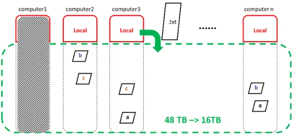
3.2 Big Data Storage and Management ... 25
3.2.1 Distributed File System (DFS) ... 26
3.2.2 Hadoop Distributed File System (HDFS) ... 26
3.2.3 MapReduce Programming ... 28
CHAPTER 4. LONG-TERM SPEED PREDICTION USING ADVANCED
CONVOLUTIONAL NEURAL NETWORK ... 37
4.1 Introduction ... 37
4.2 Methodology ... 38
4.2.1 ANN ... 38
4.2.1.1 The Basic Building Block ... 38
4.2.1.2 Understand the Capability of ANN ... 40
4.2.1.3 How to Train an ANN ... 41
4.2.1.3.1 Gradient descent ... 42
4.2.1.3.2 Backpropagation and learning rate ... 44
4.2.1.3.3 Activation function and batch ... 46
4.2.1.4 How to select the trained weights of an ANN ... 47
4.2.2 CNN ... 48
4.2.3 Proposed CNN ... 50
4.2.3.1 Encoder for Predicted Weather ... 53
4.2.3.2 Encoder for Historical Speed ... 54
4.2.3.3 Decoder ... 56
4.3 Case Study ... 57
4.3.1 Model Input ... 57
4.3.2 Model Training ... 57
4.3.3 Testing Results and Discussion ... 59
CHAPTER 5. SHORT-TERM SPEED PREDICTION USING HYBRID DEEP NEURAL NETWORK ... 64 5.1 Introduction ... 64 5.2 Methodology ... 66 5.2.1 RNN ... 66 5.2.2 LSTM ... 68 5.2.3 Proposed Hybrid LSTM ... 69 5.3 Case Study ... 71 5.3.1 Model Input ... 71 5.3.2 Model Training ... 71
5.3.3 Testing Results and Discussion ... 72
CHAPTER 6. CONCLUSIONS ... 78
REFERENCES ... 82
LIST OF FIGURES
Page
Figure 1.1 Sample speed heatmap ... 2
Figure 2.1 Deep learning trend in transportation research ... 18
Figure 3.1 Sample raw data from Wavetronix sensor ... 24
Figure 3.2 Sample raw weather data from IEM ... 25
Figure 3.3 DFS structure ... 26
Figure 3.4 HDFS storage strategy ... 27
Figure 3.5 HDFS splitting and duplication ... 28
Figure 3.6 MapReduce programming process ... 28
Figure 3.7 Locations of Wavetronix sensors along I-235 eastbound ... 30
Figure 3.8 Raw speed data in 1-minute aggregation ... 30
Figure 3.9 Smoothed speed data in 1-minute aggregation ... 32
Figure 3.10 Speed data for test day 1. ... 34
Figure 3.11 Speed data for test day 2 ... 35
Figure 3.12 Speed data for test day 3 ... 35
Figure 4.1 One-node ANN structure ... 39
Figure 4.2 Fully connected deep ANN ... 40
Figure 4.3 Simplified ANN for backpropagation illustration ... 44
Figure 4.4 Fully connected layer and CNN layer ... 48
Figure 4.5 Two-dimensional CNN layer ... 49
Figure 4.6 Proposed CNN ... 51
Figure 4.7 Structure of encoder for predicted weather ... 53
Figure 4.9 Structure of decoder ... 56
Figure 4.10 Model results on test day 1, 12-02-2016 Friday ... 61
Figure 4.11 Model results on test day 2, 12-05-2016 Monday ... 62
Figure 4.12 Model results on test day 3, 12-16-2016 Friday ... 63
Figure 5.1 Traditional NN structure for sequence prediction ... 67
Figure 5.2 Recurrent NN structure for sequence prediction ... 67
Figure 5.3 LSTM NN structure ... 68
Figure 5.4 Proposed hybrid LSTM model structure ... 69
Figure 5.5 1-D convolutional filter for feature extraction for LSTM cell input ... 71
Figure 5.6 Model results on test day 1, 12-02-2016 Friday ... 75
Figure 5.7 Model results on test day 2, 12-05-2016 Monday ... 76
LIST OF TABLES
Page
Table 2.1 Number of literatures in deep learning and speed prediction ... 18
Table 3.1 Weather variables description ... 32
Table 3.2 Statistic summary for all traffic and weather data ... 33
Table 3.3 Statistic summary for test day 1 ... 34
Table 3.4 Statistic summary for test day 2 ... 35
ACKNOWLEDGMENTS
I would like to thank Dr. Sharma for his support and guidance all these years; my co-major professor, Dr. Sarkar; and my committee members—Dr. Dong, Dr. Savolainen and Dr. Hegde—for their guidance throughout this research.
I would also like to thank my friends and colleagues who helped me during the research work at InTrans.
In addition, I would like to express my appreciation to my parents for their support. And special thanks to my wife, Tingting, who is always supporting me in my research and my life.
ABSTRACT
The objective of the proposed study is to predict traffic speeds at a route level so that the traffic management has a chance to operate proactively. A distributed file system and parallel computing platform is used to store the big data sets of statewide traffic and weather data in a fault-tolerant way and process the big data in a timely manner. Traffic speed prediction problem is studied at two levels, and two deep networks are proposed accordingly: a fully convolutional deep network for long-term speed prediction and a hybrid long short-term memory (LSTM) network for short-term speed prediction. The fully convolutional deep network utilizes both weather information and historical traffic speeds to make long-term traffic speed predictions, and a trained model can be
transferred to predict traffic speed at any spatial-temporal scale. The hybrid LSTM network utilizes the previous traffic speeds on the current day as well as historical traffic speeds to make short-term speed predictions, and a trained model can be used to predict speeds at any timestamps ahead in a streaming fashion. The proposed long-term and short-term traffic speed prediction models can be combined as a multilayer decision supporting system to provide traffic management an opportunity to operate proactively.
CHAPTER 1. INTRODUCTION 1.1 Background
Transportation systems aim to move people and goods safely and efficiently; thus, the system mobility becomes a great concern for both agencies and road users. In urban traffic systems, congestion is a major harm to mobility, which can also result in a total of $78 billion of societal and energy costs in the United States (TTI, 2007). One way to alleviate the congestion is to provide accurate and reliable traffic information and predictions, which can help both traffic planners and travelers to change plans for an alternative route in advance. Therefore, there is a need for research on how to produce an accurate understanding and reliable forecasting of traffic conditions, especially traffic speed.
With lots of intelligent transportation system (ITS) technologies being applied, large-scale, multisourced and high-resolution traffic data are available to researchers. In Iowa, enormous data can be obtained statewide from multiple sources, including roadside radar sensors, the private sector, a road asset management system (RAMS), and a road weather information system (RWIS). How to understand those massive data in an efficient way becomes a critical research task.
In recent decades, the emergence of big data technology and successful
implementation of neural network algorithms provide the opportunities to conduct data-driven research in transportation. Moreover, the innovation of a parallel computing platform makes graphics processing unit (GPU)-accelerated computing available, which brings deep learning algorithm into reality. Some deep learning algorithms, like convolutional neural network (CNN) and long short-term memory (LSTM), have the powerful ability to explore massive, heterogeneous data and make predictions. All these advances in artificial
intelligence provide researchers the chance to learn the features from traffic data in a fast and deep way. Thus, predicting the traffic speed in both the short and long term through massive, heterogeneous traffic data could be improved by using big data and deep learning approach.
1.2 Research Motivation
Traffic speed predictions studied in this dissertation are to provide agencies and road users an estimation of roadway traffic speed in the coming future by using deep networks trained on large-scale historical data.
In traffic operations and management, heatmaps have been widely used to visualize traffic speeds at a route level. A traffic speed heatmap puts speed values in a
two-dimensional array. The 2-D array typically arranges roadway sensors or monitored roadway segments along the vertical axis, expands the time along the horizontal axis, and colors each cell from green to red by the value of traffic speeds. A typical traffic speed heatmap is illustrated in Figure 1.1.
Figure 1.1 Sample speed heatmap
As shown in the illustration, traffic speed heatmaps are plots that can provide meaningful traffic speed visualization both spatially and temporally. Because of the matrix nature, the colorful 2-D plots of traffic speeds on a route level can be viewed as images. In a live traffic monitoring system, these traffic speed images are rolling along the temporal axis and the displayed images are always behind the current timestamps because of data
processing and communication latency. In this context, traffic speed prediction is basically sneak-peeking the traffic speed images beyond the current timestamp.
From the traffic operation perspective, public agencies like the Department of Transportation (DOT) would be interested in traffic speed predictions at different temporal scales.
• Long-term: A good traffic speed estimation of the next day could make DOT operators well prepared and operational strategies can be planned in advance for the potential upcoming congestions.
• Short-term: A good traffic speed estimation of the next few minutes could give traffic operation officers an opportunity to prepare for the low-speed events proactively. Traffic incident management (TIM) may take this opportunity to relocate highway helpers in advance.
Thus, a good traffic speed prediction could provide traffic operations extra
information as reference and potentially improve the reaction speed of TIM for incidents and enhance the mobility and safety of the roadway system overall.
Agencies would also be interested in traffic speed predictions at different spatial scales. The future traffic speed estimate at a certain sensor location would be useful for traffic monitoring at a targeted area, but a speed prediction of a roadway network can provide a better sense of a whole picture and thus be more useful.
Roadway users can benefit from the traffic speed prediction as well. The estimated travel speed in the next day can help drivers plan their travel time accordingly and choose an appropriate detour if applicable, and the network traffic loads can be more balanced.
on the road and before leaving better informed and help them make better adjustments from both user optimal and system optimal perspectives, thus the overall traffic congestion level on the network can be alleviated.
1.3 Problem Statement
There are several challenges in predicting traffic speeds. First is efficiently managing the large-scale, high-resolution, and heterogeneous data. Traditional databases could deal with a certain amount of multivariate data but require excessive time and memory, which is a main obstacle in data-driven research.
The second is the high computational complexity requested by predicting traffic speeds. Traffic speeds on a network have both spatial and temporal correlations that make them challenging to predict. Although there have been lots of prediction models available, the traditional methods still lack the capability to deal with high computational complexity.
To provide accurate predictions to travelers and planners, both short-term and long-term predictions should be considered. Current methods tend to treat speed data as a time-series and have less prediction power, especially in long-term prediction. They also have limited ability in exploring heterogeneous data in a scalable manner. This research aims to solve these problems by answering the following research questions:
1. How to apply big data technologies to efficiently integrate massive traffic data?
2. How to predict short-term speeds at a route level? 3. How to predict long-term speeds at a route level?
1.4 Research Objective
According to the different use cases and different technologies required, this
long-term prediction, which estimates traffic speeds in the next few hours or even the next day; and (2) short-term prediction, which estimates traffic speed in the next few minutes. In both long-term and short-term prediction cases, this dissertation applies deep neural network models that can be trained on historical data collected from various sensors with no manual labeling needed and estimate future traffic speeds at a route level. The research objectives are the following:
1. Develop database to store, integrate, and analyze big traffic data.
In this research, the raw streaming traffic data from roadside radar sensors (Wavetronix) and weather data provided by Iowa Environmental Mesonet (IEM) are
downloaded and stored in a distributed way. A parallel processing method will be introduced and applied to those data.
2. Predict long-term speed to provide big picture traffic conditions to traffic planners.
The long-term speed prediction discussed in this dissertation is predicting the traffic speeds of the next few hours or the next day at a route level. The prediction model should take advantage of the large amount of historical data. The pretrained model should provide high transferability for deploying on different roadway networks and predict speeds in the desired time scale.
3. Predict short-term speed to provide advance traveler information.
The short-term speed prediction discussed in this dissertation is predicting the traffic speeds of the next few minutes at a route level. Unlike the long-term traffic speed prediction that usually is done once in a while, the short-term traffic speed prediction should be done in a streaming fashion.
1.5 Dissertation Organization
This dissertation consists of six chapters including an introduction. Chapter 2 presents a comprehensive literature review on current predictive analysis and artificial intelligence in transportation. Chapter 3 describes the database built on multiple data sources using big data technology. According to the complexity level of the methodology used, the long-term prediction will be discussed first then the short-term prediction will follow. Chapter 4 presents the prediction of long-term traffic speed at a route level using a fully convolutional deep network. Chapter 5 presents the prediction of short-term traffic speed at a route level using a hybrid LSTM network. Chapter 6 concludes the research by summarizing the findings and outlining the future work.
CHAPTER 2. LITERATURE REVIEW
This chapter presents a comprehensive literature review, focusing on the research related to traffic speed prediction and deep learning in transportation. Currently, the methods used for traffic speed prediction can be put into two general categories: statistical modeling and artificial intelligence (AI). Based on the categories, this section will review two kinds of past research on prediction and provide the background of methods employed in this study.
2.1 Statistic Modeling in Traffic Prediction
Statistical analysis has been the major method in the traffic speed prediction field for a long time, and it is still being widely used. Several kinds of methods, including
fundamental traffic flow theory, time-series models, and Kalman Filter (KF), are discussed.
2.1.1 Traffic Flow Theory
Previously, many transportation researchers relied on the flow theory to explore different stages of traffic flow and make predictions. Most of them were focusing on volume prediction by estimating the origin-destination (OD) matrix on the network (Camus et al., 1994; Crittin and Bierlaire, 2002). There are also many studies using flow theory that were implemented in simulations. Besides traffic volume estimation, researchers also tried to represent the full traffic evolution with volume, density, and speed. Daganzo (1994)
proposed a cell transmission model (CTM) to represent traffic evolution and further predict it over time and space.
Treating traffic flow as a stochastic process, some researchers have explored and modeled the stochastic characteristics in traffic flow to predict short-term speed. Qi and Ishak (2013) focused on urban freeways during peak hours and estimated the speed transition probabilities, from which the expected values were extracted and fitted using exponential
models. However, this method tends to be affected by study location and time period, which makes it less scalable.
2.1.2 Time Series Model
Since the traffic data is time variant, time-series modeling has been widely used in traffic data analysis. One typical model, autoregressive integrated moving average (ARIMA), assuming stationarity and constant variance, is often adopted in traffic prediction research. Hamed et al. (1995) and Lee and Fambro (1999) have used the ARIMA model to predict traffic volume. Further, Williams et al. (1998) and Williams and Hoel (2003) explored the seasonality by using the seasonal ARIMA (SARIMA) model. Other researchers also tried to combine generalized autoregressive conditional heteroscedasticity (GARCH) with the ARIMA model to deal with the volatility in traffic conditions (Kamarianakis et al., 2005; Chen et al., 2011).
Several methods developed on the ARIMA model for speed prediction were also explored. Cetin and Comert (2006) have proposed an adaptive ARIMA model to
accommodate regime change in traffic (such as free flow regime, congested regime, etc.). They implemented expectation maximization (EM) and cumulative sum (CUSUM) methods to detect the change in the mean of process, then applied the ARIMA model with adaptive parameters. Wang et al. (2014) combined empirical model decomposition (EMD) with ARIMA and created a hybrid EMD-ARIMA model. Emperical model decomposition
decomposed the traffic data into intrinsic model functions (IMFs), then ARIMA models were applied on each of the IMFs, and finally the components were reconstructed to the predicted traffic speed.
To capture the spatial relationship existing in traffic flow, many researchers have been working on multivariate time-series analysis. Williams (2001) used the ARIMAX
model to incorporate upstream volume as a transfer function input(s). Kamarianakis and Prastacos (2003) compared univariate and multivariate models for traffic prediction. Mainly they applied the ARIMA model, the vector autoregressive moving average (VARMA) model, and the space-time ARIMA (STARIMA) model to predict the speed on major arterials. The forecasting results showed a better performance in the multivariate model, which can cope with the interdependencies between speed from neighboring detectors. Pavlyuk (2017) also compared several multivariate models, such as VARMA, error correction model (VECM), STARIMA, and the multivariate autoregressive space state (MARSS) model for speed prediction. This study found the multivariate model can capture the spatial and temporal relationship in traffic flow and suggested simultaneous modeling on volume, speed, and occupancy to improve predictions.
Similar work in traffic speed predictions using multivariate models has also been done. Chandra and Al-Deek (2008, 2009) have used the vector autoregressive (VAR) model to account for the spatial relationship with taking two upstream and two downstream
locations into consideration. And Zou et al. (2015) have proposed a hybrid model to estimate the speed series by periodic trend and residual part, with the assumption that speeds have a daily periodic trend on work days. They used the trigonometric regression function to estimate the periodic component and tried space time (ST), VAR, and ARIMA models to estimate the residual. The results showed a better performance in the hybrid ST model with different prediction steps.
Besides the ARIMA model, other multivariate methods were also explored. Ghosh et al. (2009) have proposed the structural time-series model (STM) with regard to multivariate data. This model separated components in a time-series and was used on signalized
intersections to predict traffic volume. Another improvement in multivariate time-series analysis is made by Szeto et al. (2009). They embedded CTM in the SARIMA model to achieve volume prediction on a signalized network.
Time series models are widely used in traffic prediction; however, they are still constrained by the assumption of stationary process and the linear combination of previous observations. Moreover, compared to traffic volume, traffic speed has less obvious patterns and can be impacted by latent factors, which makes it hard to be predicted by traditional time-series analysis.
2.1.3 Kalman Filter
The KF utilizes the observed measurements and current estimated state to generate the estimation of a future state with statistical noises. This state space-based model can cope with multivariate data; thus, it has been applied in many traffic prediction studies. Okutani and Stephanedes (1984) first used KF to predict short-term traffic volume and found a better performance than the benchmark model UTCS-2. Further, Xie et al. (2007) improved the volume prediction by using discrete wavelet decomposition to denoise the raw data and get multilevel data series, then applying KF to estimate the volume. The results showed the proposed wavelet KF outperformed the direct KF. Another improvement on volume prediction was made by Guo et al. (2014). They proposed an adaptive KF to update the process variance by using the observation errors and state estimation errors to fine-tune the variances and implement the Kalman recursion.
Some researchers also focused on travel time prediction. They have used KF to estimate freeway travel time using different data sources such as toll tags (Chien and Kuchipudi, 2003; Chien et al., 2003), GPS data (Yang, 2005), and inductive loops (Xia, 2006). Further, Kuchipudi and Chien (2003).provided the flexibility in choosing path-based
or link-based travel time estimation according to the traffic condition based on their previous research. Lint (2008) also proposed an extended KF (EKF) enabling online learning to predict freeway travel time. Other applications have also been done on network-level traffic prediction embedding KF (Whittaker et al., 1997; Wang et al., 2006).
Although there are lots of studies in traffic flow prediction using KF, few applications can be found in traffic speed prediction. Yang et al. (2004) have proposed an adaptive
recursive least-squares method to predict traffic speed online. They used an autoregressive (AR) model to generate an offline estimate for the transition coefficient matrix and noise covariance matrix, and they made predictions with KF online. One problem in this study is the spatial relationship has not been explored, which exists in traffic propagation.
The KF can deal with multivariate time series and update the state continuously; however, it requires the knowledge of state transition and noise covariance, which are hard to determine in traffic flow.
2.2 Artificial Intelligence in Transportation
By moving toward AI, many more techniques and tools are revealed in front of traffic researchers and engineers. The adequate data also made it possible to implement machine learning and data mining techniques to make short-term and long-term predictions of traffic flow. This section reviews several shallow machine learning algorithms and the application in traffic flow prediction, such as 𝑘-nearest neighbor (𝑘NN), support vector machine (SVM), and artificial neural network (ANN). With the emergence of deep learning, this powerful tool can also be used to predict traffic. Thus, this section will also emphasize deep learning algorithm applications in transportation and how they inspire this study.
2.2.1 Nearest Neighbor Algorithm
In data mining domain, a nonparametric, pattern matching technique, 𝑘NN algorithm, is commonly used. This method has also been adopted in transportation research. Smith and Demetsky (1996) used the nearest neighbor model to predict traffic volume in multiple intervals in advance on freeway segments. It had the advantages in scalability and ability of predicting relative long-term volume. Other than volume, Handley et al. (1998) have also proposed the 𝑘NN model to predict the travel time at multiple locations on a freeway. They examined and selected three nearest neighbor, different predictive features and normalization schemes, and from the results, they suggested that speed prediction is less accurate than volume during peak hours. Further, a hybrid model integrating geographic information system (GIS) and nonparametric regression has been developed to improve the prediction of travel time (You and Kim, 2000). In regard to multivariate traffic characteristics, Clark (2003) has predicted the traffic state by using the 𝑘NN model. The method was applied on one highway location with one month of data; it turned out to be a good prediction in flow and occupancy, but it did not perform well in speed prediction.
In previous literature, compared to traffic speed, the pattern of traffic volume—such as the peak hour pattern and seasonal pattern—seems easier to capture. Thus, this method is more often used in traffic volume prediction. Researchers have conducted many studies on predicting traffic flow (Smith et al., 2002; Zhang et al., 2013; Zhong and Ling, 2015). Efforts have also been made for a real-time system (Oswald et al. 2000; Smith and Oswald, 2003). Researchers have also tried different input variable structures to improve the prediction. Kindzerske and Ni (2007) have used a composite approach in the nearest neighbor search to predict traffic conditions. They tended to not use the whole network as input; instead, they
only chose two upstream and two downstream sensors to form a local network to make predictions in order to minimize the error.
There is little research with a focus on traffic speed prediction using 𝑘NN. One was done by Yildirim and Cataltepe (2008), which used both 𝑘NN and SVM to predict traffic speed in 5-minute intervals. The results indicated SVM has a better performance than 𝑘NN. The other speed prediction study conducted by Chen et al. (2014) integrated Gaussian process regression with 𝑘NN. They used 𝑘NN to extract data features and input them to Gaussian process regression to achieve a reliable prediction.
Overall, this method is easy to implement and transfer using simple features extracted from historical data; however, it does not outperform the more advanced machine learning techniques in terms of prediction accuracy.
2.2.2 Support Vector Machine
The SVM method or support vector regression (SVR) is one of the most currently used machine learning techniques in traffic flow prediction. Wu et al. (2004) have used SVR to predict travel time on a highway network with three different kernel functions examined. The results performed better than the baseline prediction the authors selected. Other
researchers also have applied SVM on travel time prediction and compared the root mean square error (RMSE) with other baseline models (Yu, Yang and Yao, 2017; Vanajakshi and Rilett, 2007).
Since SVM is a powerful tool in traffic prediction, there are many researchers who have added extra techniques to improve the model performance from solely using SVM. Asif et al. (2014) clustered the traffic data by unsupervised learning methods based on their spatiotemporal patterns before applying SVR, and it benefits the prediction results. One
advantage of SVR is that it allows a kernel function to implicitly boost the input features up to a higher dimension, but choosing the right kernel function can be a trial-and-error process. Wang and Shi (2013) constructed a new kernel function in SVR using a wavelet function to capture the nonstationary characteristics of the short-term traffic speed data and report better performance over traditional SVR. Although SVR with kernel function overcomes the linear constraints, the model performance is highly relied on for the engineered input features.
Furthermore, there are many variants of SVR, such as least squares SVM (Zhang and Liu, 2009), 𝑣-SVM (Zhang and Xie, 2007), online-SVR (Castro-Neto et al., 2009), and seasonal SVR (Hong, 2011), which focused on different aspect of traffic flow prediction, such as travel time, traffic volume, etc. Also, to capture the spatial and temporal relationship in traffic flow, Li et al. (2016) have combined the ARIMA model and SVR to generate a hybrid strategy to predict highway volume in a more accurate and stable way. Besides those SVR variants with focus on prediction, Gopi et al. (2013) have proposed a Bayesian SVR to focus on the error variation of predicted traffic speeds.
Support vector machine can be a powerful tool in prediction; however, it mainly relies on the pattern of historical data and has shortcomings in exploring the temporal relationship, which is a nature of traffic speed data.
2.2.3 Artificial Neural Network
One great aspect of the neural network (NN) is that it can mimic any function by stacking tons of parameters in a simple way, and the useful features are automatically extracted through the training process. This method has been applied in traffic prediction increasingly in recent years.
One typical NN often refers to the back propagation NN (BPNN). The idea for back propagation is that inputs are fed forward to the network and then errors between output and
target are propagated backwards through the network; meanwhile the weights are updated by some optimization technique. The BPNN was applied in traffic volume prediction as early as the late 90s (Kwon and Stephanedes, 1994; Smith and Demetsky, 1994; Yun et al., 1998). In terms of traffic speed prediction, Huang and Ran (2003) have investigated the traffic speed under adverse weather using BPNN for a single link. They used weather and traffic variables as inputs and built a fully connected NN. Lee et al. (2007) took the time of day and day of week into account. Other researchers also used the ANN to predict traffic speed and
compared it with traditional ARIMA or a pattern matching model (Lee et al., 2006; Fabritiis et al., 2008; Park et al., 2011; Ye et al., 2012; Habtie et al., 2017).
Based upon the NN concept, much improvement has also been accomplished. One improvement is focusing on the network structure optimization. Researchers used a genetic algorithm to determine layer connection or nodes (Abdulhai et al., 1999; Lingras and Mountford, 2001; Wang et al., 2005; Vlahogianni et al., 2005). Some researchers also
focused on preprocessing the traffic data to achieve a better prediction performance. Park and Rilett (1998) explored two clustering techniques—Kohonen self-organizing feature maps and fuzzy c-means model—to extract features from data before they were fed it into the NN. Jiang and Adeli (2005), Xie and Zhang (2006), and Boto-Giralda et al. (2010) used wavelet transform to denoise the data for network training and made predictions on traffic volume.
Inside the NN, some researchers also tried to replace the sigmoid function in hidden layers with radial basis function (RBF). They have employed this model to predict traffic volume and compared it with other methods (Amin et al., 1998; Park et al., 1998; Xie and Zhang, 2006; Zheng et al. 2006; Chen, 2017; Li et al. 2017). This kind of NN has a simple
structure and is fast to learn. But the performance relies on the center and width parameter estimation of the RBF.
Different NNs could be applied on different traffic conditions. Park and Rilett (1998) proposed a modular NN by first clustering the data and then building a modular NN for each classification. This approach could estimate the entire function separately without the
requirement of prior knowledge like other function approximation schemes. Similarly, Chen et al. (2001) used a self-organizing map (SOM) to cluster the traffic data and then used BPNN for each cluster. Lee (2009) used the k-means clustering method before predicting the travel time using ANN. This concept has also been adopted by other researchers (Yin et al., 2002; Coufal and Turunen, 2003; Tang et al., 2017). They tended to cluster the input data by fuzzy approach and apply the NN to each group with a similar traffic pattern.
To cope with the nature of time dependency in traffic data, many researchers have improved the NN structure with a recurrent feature. Some recurrent neural networks (RNNs) with context units to remember the previous output have been applied, such as the recurrent Jordan networks to forecast traffic volume (Yasdi, 1999), the recurrent state-space NN to predict travel time (Lint et al., 2002), a time-lagged recurrent network to predict short-term traffic speed (Dia, 2001). Ishak et al. (2003) explored three different networks for speed prediction—Jordan-Elman networks, partially recurrent networks, and time-lagged feedforward networks—and tried to optimize the network performance by using different input settings. Similar works have also been done by Zeng and Zhang (2013) and Jiang et al. (2016), which compared different RNN topologies on traffic speed and travel time
Some hybrid models have been explored by embedding statistical modeling in ANNs (Zeng et al., 2008; Moretti et al., 2015). Zheng et al. (2006) have also tried to combine two types of NN (BPNN and RBFNN) by using the Bayesian approach. The results showed it performed better than the single predictor. In addition, Alecsandru and Ishak (2004) have explored various topologies of the NN model to test the performance in traffic flow prediction.
The advantage in the ANN family algorithm is the capability in handling complex, nonlinear relationships in multivariate data. In terms of time-series prediction, however, the traditional NN is limited by short-term memory, which neglects the long-term trend that exists in a speed sequence. Also, a traditional ANN also has a limited structure due to the computational power constraint before GPU-accelerated computing was in place.
2.2.4 Deep Learning
2.2.4.1 Deep Learning Trend in Transportation Research
The deep learning concept was introduced back in the 80s and developed increasingly since the breakthrough in 2006 made the training fast and effective (Hinton and
Salakhutdinov, 2006; Hinton et al., 2006). Transportation researchers have also adopted the deep learning algorithm in recent years. Some advanced deep models like the CNN and LSTM have been used for traffic prediction. Table 2.1 lists the number of literatures in deep learning (with CNN and LSTM highlighted) in the general transportation area and the traffic speed prediction with deep learning.
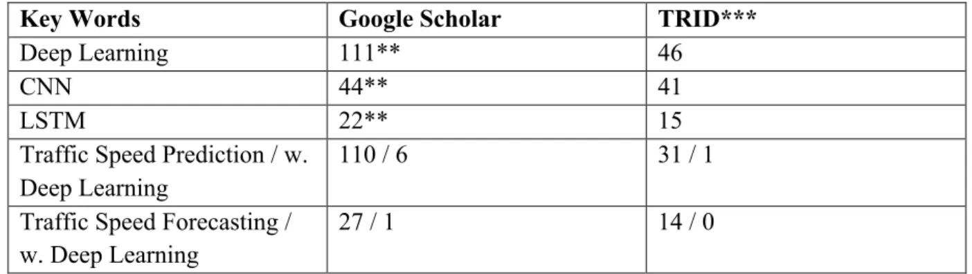
Table 2.1 Number of literatures in deep learning and speed prediction*
Key Words Google Scholar TRID***
Deep Learning 111** 46
CNN 44** 41
LSTM 22** 15
Traffic Speed Prediction / w. Deep Learning
110 / 6 31 / 1
Traffic Speed Forecasting / w. Deep Learning
27 / 1 14 / 0
* As of 3/10/2018
** With additional key words “traffic” or “transportation”
*** TRID is an integrated database that combines the records from the Transportation Research Information Services (TRIS) database and International Transport Research Documentation (ITRD) Database. TRID provides access to more than one million records of transportation research worldwide.
Figure 2.1 also shows the trend of deep learning in transportation research. Notably, the peak is the last Transportation Research Board (TRB) annual meeting, with many researchers presenting their studies. Deep learning has gained more and more attention, which motivates this study in speed prediction as well.
2.2.4.2 Deep Belief Network
In traffic flow prediction, the first application is made by Huang et al. (2014) using deep belief networks (DBNs) to predict traffic volume from a single location and multiple locations (with multitask learning). Unlike the deep neural network (DNN), DBN has undirected connections in layers, which can be treated as stacked restricted Boltzmann machines (RBMs) and trained layer by layer as unsupervised. Huang et al. (2014) utilized DBN architecture and further added a multitask regression layer to predict volume with supervision. The results outperformed shallow machine learning models. Similar studies have also been done. Jia et al. (2016) used DBN to predict traffic speed; Tan et al. (2016)
compared different RBM settings in the DBN for volume prediction. In addition, Lv et al. (2015) used stacked auto-encoders (SAE) with unsupervised greedy layer-wise training to predict traffic flow.
2.2.4.3 Deep Neural Network
Some researchers have worked on developing traditional ANN into deep learning. A simple DNN was applied by Yi et al. (2017) predicting the traffic performance index from speed data. Another structure adopted from image processing is CNN, which has the
advantages in dealing with spatial relationship as it maintains the spatial correlation through convolution. By treating multiple location speed sequences as images, Ma et al. (2017) applied deep CNN to predict the speed image in the next 10 and 20 minutes. However, one important problem in this approach is that the network is not fully convolutional. The last several fully connected layers may potentially lose the structural dependencies maintained throughout the previous CNN layers, and the full connection limits the model inputs to a fixed size; thus a pretrained model cannot be directly applied on another roadway segment.
2.2.4.4 Deep Recurrent Neural Network
Due to the nature of time dependency in traffic data, some studies have been
conducted with focuses on recurrent model structure. Ma et al. (2015a) combined RBM with RNN to predict a binary congestion condition on the roadway network. Wang et al. (2016) used CNN with an error-feedback recurrent layer to predict traffic speed. After using the convolution layer to extract the features, they applied a recurrent layer containing both regular neurons and error-feedback neurons to capture the incidents that can cause speed pattern change.
Although RNN aims to capture the pattern in time series, in practice it has a big problem—it is not good at capturing long-term dependencies. To overcome the long-term memory loss, a new structure has been developed. Long short-term memory has been introduced by Hochreiter and Schmidhuber (1997) and increasingly used in time-series prediction. Ma et al. (2015b) applied an LSTM model that is a special type of RNN for traffic speed prediction. With the speed, volume, and occupancy of one sensor as input and the speed in the next 2 minutes as output, the author demonstrated the efficiency of DNN, but a lot more potentials of DNN have not been excavated. Chen et al. (2016) used LSTM to classify and predict the categorized traffic conditions (congested, slow, free flow). Duan et al. (2016) trained LSTM models for each roadway segment using travel time series data, and they predicted a travel time vector four steps ahead. The LSTM model achieved relatively higher accuracy in first step prediction. However, they predicted each location on the same highway independently; thus the spatial dependencies are not utilized. Fu et al. (2016) applied both LSTM and a gated recurrent unites (GRU) model to predict traffic volume in 5-minute intervals. The GRU has a simpler structure than LSTM, which can potentially reduce the computation time. They randomly selected 50 locations from a traffic network and used
previous 30-minute data to predict the next 5-minute volume. The results showed LSTM and GRU outperformed the traditional ARIMA model. Jia et al. (2017) integrated rainfall data to predict traffic speed using DBN and LSTM. To take the spatial correlation into account, Zhao et al. (2017) included the data from other locations as the input of the LSTM unit at the target location. They used traffic volume data in 5-minute intervals and predicted up to a 60-minute volume. In order to capture the backward temporal dependency, Cui et al. (2018) used a bidirectional LSTM model. They used speed data in 5-minute intervals and tested different numbers of steps in spatial and temporal input. The results indicated stacking one bidirectional LSTM layer and one unidirectional LSTM layer performed the best in the experiments compared to other architectures. One limitation is the lack of historical speed information as inputs so that the seasonal or periodical characteristics of traffic may not be captured. In addition, “backward temporal dependency” in the prediction problem itself may be arguably a nonvalid term, so that the need of bidirectional LSTM is questionable.
2.2.4.5 Hybrid Deep Learning
With the advance of CNN in spatial feature extraction and LSTM in temporal feature extraction, some studies have been conducted to learn the feature from spatiotemporal correlated traffic data by assembling two models. Wu and Tan (2016) combined CNN and LSTM to predict traffic flow. They proposed the model with one CNN layer, two LSTM layers, and one fully connected layer. The results showed a lower mean absolute error (MAE) compared to the single LSTM model. Similar work has also been done by Yu et al. (2017). They used CNN to learn the spatial features and LSTM to learn the temporal features. One improvement occurred when preparing the training data—they represented the road network in grid to retain the structure. Liu et al. (2018) also used CNN to extract features and
architecture such as tuning the number of LSTM layers, number of DNN layers, etc. They proposed one CNN layer plus two LSTM layers plus two DNN layers is the best structure in the predictions on different horizons and using different sliding inputs.
Deep learning is prevailing in transportation research as we are getting large-scale, high-resolution, and multisource traffic data. Deep learning has the advantages in exploring dynamic and implicit correlation in data with less assumptions and prior knowledge. But deep networks need to be driven by a large amount of data and the impact of a certain feature could not be easily explained.
2.3 Summary
Numerous studies have been done in traffic prediction, from exploration in
fundamental traffic flow theory, time series modeling, to artificial intelligence applications. Prediction is still a tough task to complete. In past research, most traffic prediction focuses on volume prediction rather than speed prediction. One reason could be traffic speed has less obvious trends (peak hour, weekday/weekend) than traffic volume. Also, volume is
determined by traffic demand and supply; however, speed can be less sensitive to volume if demand is served. On the other hand, speed can be sensitive to other factors such as weather condition, incident occurrence, etc., that sometimes are unobserved. These properties in traffic speed result in a harder prediction.
Among all the reviewed studies, a true long-term speed prediction like daily speed profile prediction is still not investigated. Forecasting daily speed profiles can benefit traffic planners in preparation for any weather hazards impacting traffic or for congestion relief measures planning.
CHAPTER 3. BIG DATA IN TRAFFIC DATABASE DEVELOPMENT
High-volume, high-resolution, heterogeneous traffic data can be obtained or accessed today by many transportation agencies. How to store, manage, and utilize these data is important. With the advent of big data technology, a solution is developed to efficiently manage the traffic database. In this chapter, the database developed for statewide traffic data management using big data techniques is discussed. The contents include (a) data acquisition, (b) big data storage and management, and (c) data preprocessing, particularly for this speed prediction research.
3.1 Data Acquisition
The Iowa DOT deploys more than 500 roadside radar sensors and 700 cameras, including both permanent and temporary versions statewide. Permanent sensors and cameras are typically located within major metropolitan areas in the state, while the temporary
versions are commonly used at locations where a work zone is present. Traffic data collected by Wavetronix radar sensors stream to a web server, and the ITS vendor manages and
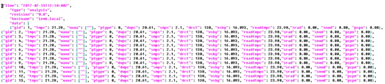
disseminates them to the Iowa DOT via secured uniform resource locators (URLs). This implementation gives us the capability to perform real-time processing and application. Data are accessible in a not well-structured extensible markup language (XML) format, which requires a parsing program using more flexible languages than structured query languages (SQLs) in traditional database management. A sample of raw data we received is illustrated in Figure 3.1.
Figure 3.1 Sample raw data from Wavetronix sensor
Traffic data collected include traffic volume, average speed, sensor occupancy, vehicle classification, and sensor status (operational, failed, off) every 20 seconds. Such high resolution and large-scale data requires big data tools to store and parallel processing to manage.
Along with Wavetronix data, weather information collected from the IEM in the observing networks is also available. Different from sensor data that are streaming, weather data are stored on a server every five minutes by the IEM team. A sample of raw weather data is illustrated in Figure 3.2. We download and parse the json file into a comma-separated value (CSV) file and store it on our local machine. Since the weather data are in five-minute resolution and cover the whole state of Iowa with small grids (rectangular longitude and latitude grids at a resolution of 0.01 degrees in both directions), it results in an enormously large amount of data that cannot be accessed by any traditional tools (more than
precipitation, wind speed, etc. Selected variables are used for traffic speed prediction, which will be discussed in section 3.3.
Figure 3.2 Sample raw weather data from IEM
Since the access methods for traffic and weather data are different, different data acquisition techniques and programs are implemented. Traffic data are downloaded and migrated to our file system through a real-time processing Java program and weather data are downloaded and parsed in Java in a batch processing. The traffic data acquisition program is written in multithread fashion. It is running on the high-performance cluster (HPC) to download the XML from the webpage every 20 seconds. The program allows the data downloading processes to be executed independently in parallel. This handles the potential timing-out issues in the web service connection and ensures that the data can be downloaded smoothly. The downloaded XML data is further parsed and then appended into a CSV formatted file for better data structure and storage saving.
3.2 Big Data Storage and Management
The streaming traffic data accumulate to more than 15 GB monthly and batch weather data are more than 140 GB monthly. An enormous amount of data requires a large-capacity, fault-tolerant, and fast-processing database. The database should hold all the data from multiple sources as their raw format so that no information is lost and new analysis can be potentially applied on any historical data at any time point. These directly lead to a big data tool for data storage and management.
3.2.1 Distributed File System (DFS)
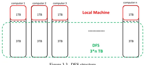
A DFS is a model in which components located on networked computers
communicate and coordinate their actions by passing messages. In other words, a DFS is a cluster of computers in which each computer within the cluster interacts and coordinates with each other to achieve a common goal as a whole. An illustration of the DFS structure is shown in Figure 3.3.
Figure 3.3 DFS structure
A DFS can be easily expanded by adding more computers into the cluster so that it is scalable and can handle big data sets. On a DFS, distributed processing can be applied on big data sets, which normal file systems can hardly handle. In distributed processing, a certain data processing job can be split into multiple components and all the components are executed in parallel by different processing units. With this distributed processing fashion, not only can a big data set be processed with limited amounts of memory, but the time it takes to process a certain job is significantly reduced.
3.2.2 Hadoop Distributed File System (HDFS)
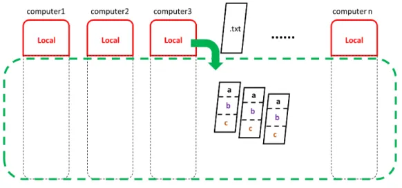
There are various software frameworks used to operate a DFS and run distributed processing jobs on very large data sets. In our case, Apache Hadoop was selected because it is open source and can be installed on computer clusters built from commodity hardware. In
an HDFS, a big dataset is split into multiple smaller chunks and each chunk is duplicated several times with each duplicate being stored on a different computer within the cluster. An illustration is shown in Figure 3.4. This way of splitting makes it possible to store a big data set with a size larger than the storage on a single computer and the duplication makes the system robust to hardware failures.
Figure 3.4 HDFS storage strategy
The HDFS itself controls the level of splitting and duplication to optimize the system performance and handles the addressing between chunks behind the scenes so the user is not bothered by these lower-level communications when using the HDFS. In this study, 14 computers with 6 terabyte (TB) storage each were built as an HPC. Half the storage from each computer was configured into the HDFS. The remaining half storage was preserved for local usage. The final configured HPC consists of 14 computers with 3 TB local storage on each and a 42 TB HDFS. An illustration is shown in Figure 3.5.
Figure 3.5 HDFS splitting and duplication
3.2.3 MapReduce Programming
MapReduce is the basic framework for distributed processing in an HDFS. It parcels out work to various processing units called nodes within the cluster, then organizes and reduces the results from each node into a cohesive answer to a query. MapReduce utilizes the key value pair to distribute the data as programmed. Different data but with the same key will dump into one reducer to process. A brief process inside MapReduce programing is shown in Figure 3.6. MapReduce works very efficiently in many frequently performed jobs of traffic data processing such as filtering, grouping, data aggregation, etc.
There are more than 5 million records (rows) of traffic data in the raw CSV file of a single day. EXCEL is not capable of processing data of a single day because of the 1 million row limit, and MATLAB, R, or other traditionally used tools can be annoyingly slow. As a comparison, the distributed computing under the MapReduce framework is super-fast and scalable to larger datasets. In the HDFS, a sequence of filtering, grouping, and aggregating tasks can be done on one-day data in several seconds, on one-week data in a minute, and on one-year data in approximately half an hour.
In our study, the 20s raw data needed to be re-aggregated into larger time bins for model training. MapReduce programs were written in Java and executed to process the big datasets stored in the HDFS.
3.3 Preprocessing for Speed Prediction Analysis
For the speed prediction case study, the eastbound traffic data collected by 15 Wavetronix sensors on Interstate 235 (I-235) were used. Figure 3.7 displays the locations of the 15 traffic sensors. The 15 sensors covered an 11-mile-long corridor located in the center of the Des Moines metropolitan area. To cover this area, weather information from 15 corresponding grids were used. Traffic and weather data collected from September 2015 to the end of 2016, 447 days in total, were used for both the long-term and short-term traffic speed prediction case study.
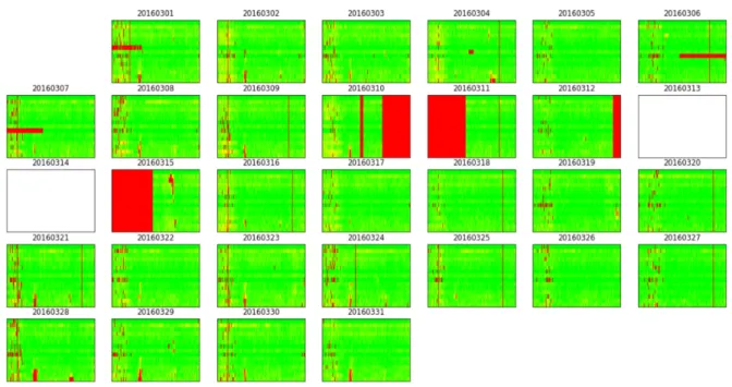
Figure 3.7 Locations of Wavetronix sensors along I-235 eastbound The traffic and weather data are arranged in image-like 2-D arrays by time and location as described before. Because of connection failures or sensor errors, there are missing data as well as wrong data involved in the raw data collected directly from sensors. Therefore, data filtering and smoothing are needed before any analysis. Figure 3.8 shows a speed calendar plot of the raw traffic speeds re-aggregated in 1-minute intervals in March 2016.
Each subplot is a 1-day traffic speed heatmap with the 15 sensors ordered by location along the vertical axis and time of day along the horizontal axis. Each traffic speed heatmap is a 15x1440 2-D array. The red patches spreading a whole column are missing data usually caused by connection failures. The narrow red bands spreading horizontally are missing data due to a single sensor malfunction or temporal shut-down. Some other sparse red dots are possibly caused by sensor errors. A day is left blank if the whole day’s data is completely missing. The data filtering and smoothing is performed in two steps.
1. Fill the missing data by the average of data from the same sensor, same time of day, and same day of week in other weeks.
2. Smooth the data of each sensor by moving the average with a 5-minute
window size.
Note that the method for filling missing data used here may not be the best strategy. In addition to averaging by sensor location, time of day and day of week, averaging by more detailed weather conditions such as by snow versus no snow may better retain the dynamics in data and provided better modeling results. But considering the fact that the missing data is relatively a small potion (5.6%) and the conditional averaging strategy can go very deep itself involving study on significant impact factors, the data smoothing method used here sticks to the simple strategy.
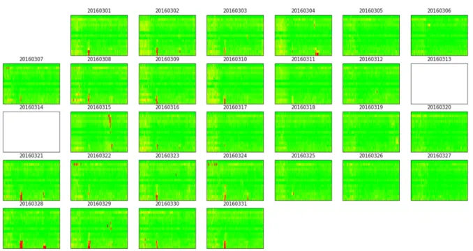
The speed calendar plot of March 2016 after data filter and smoothing is shown in Figure 3.9. Besides traffic speeds, traffic information includes vehicle count and sensor occupancy as well. Weather information contains 9 variables listed in Table 3.1.
Figure 3.9 Smoothed speed data in 1-minute aggregation Table 3.1 Weather variables description
Variable Description Measure Details
tmpc Temperature Two-meter above ground level air temperature. This value would be over a typical landscape for the location and not necessarily concrete, except in very urban areas. Units are Celsius.
dwpc Dew point temperature
Two meters above ground level dew point temperature. As with “mpc,” the same landscape assumptions apply. Units are Celsius. smps Wind speed Ten meters above ground level wind speed. This speed does not
include gusts, but is averaged over a couple-of-minutes period. Units are meters per second.
drct Direction Wind direction, where the wind is blowing from, at ten meters above ground level. Units are degrees from North.
vsby Visibility Horizontal visibility from automated sensors. Units are kilometers. roadtmpc Road
temperature
Pavement surface temperature derived from available RWIS reports. These reports include both bridge and approach deck temperatures. Units are Celsius.
srad Solar radiation
Photoactive global solar radiation, sometimes called “shortwave down”. Units are watts per meter squared.
snwd Snow depth Snowfall depth analyzed once per day at approximately 7 AM local time. If the reported snowfall depth was zero at 7 AM and it started snowing at noon, this field would still be zero until it updated the next day at 7 AM. Units are millimeters.
pcpn Precipitation 5-minute precipitation accumulation ending at the time of analysis. This is liquid equivalent. Snow and sleet are melted to derive this value. Units are millimeters accumulated in 5 minutes.
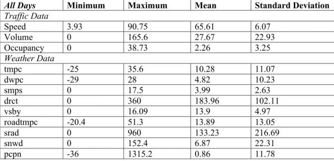
There are 5.6% of traffic data is missing and 0.0% of weather data is missing. Table 3.2 shows the summary statistics of the data after the preprocessing in the total 447 days.
Table 3.2 Statistic summary for all traffic and weather data
All Days Minimum Maximum Mean Standard Deviation
Traffic Data Speed 3.93 90.75 65.61 6.07 Volume 0 165.6 27.67 22.93 Occupancy 0 38.73 2.26 3.25 Weather Data tmpc -25 35.6 10.28 11.07 dwpc -29 28 4.82 10.23 smps 0 17.5 3.99 2.63 drct 0 360 183.96 102.11 vsby 0 16.09 13.9 4.97 roadtmpc -20.4 51.3 13.89 13.05 srad 0 960 133.23 216.69 snwd 0 152.4 6.87 22.31 pcpn -36 1315.2 0.86 11.78
Three days are selected for testing purposes in both long-term and short-term predictions.
1. Test day 1: 12-02-2016 Friday. Nonrecurrent congestion on I-235 west end
during PM peak hours. A comparison of average traffic speeds against test day 1 is shown in Figure 3.10. The data summary statistics of test day 1 are shown in Table 3.3.
2. Test day 2: 12-05-2016 Monday. Recurrent congestions on I-235 west end
during both AM and PM peak hours and nonrecurrent congestion on I-235 east end during PM peak hours. A comparison of average traffic speeds against test day 2 is shown in Figure 3.11. The data summary statistics of test day 2 are shown in Table 3.4.
3. Test day 3: 12-16-2016 Friday. Nonrecurrent congestion on I-235 west end during AM peak hours and big congestion on the whole segment during PM peak hours. A comparison of average traffic speeds against test day 3 is shown in Figure 3.12. The data summary statistics of test day 3 are shown in Table 3.5.
Figure 3.10 Speed data for test day 1. Table 3.3 Statistic summary for test day 1
Test Day 1 Minimum Maximum Mean Standard Deviation
Traffic Data Speed 27.12 85.03 65.04 5.81 Volume 0 117.8 16.59 22.77 Occupancy 0 34.7 1.36 2.4 Weather Data tmpc 0 28 21.15 6.44 dwpc 0 20 15.98 4.44 smps 0 5.7 2.71 1.47 drct 0 300 150.28 45.39 vsby 0 16.09 14.96 4.03 roadtmpc 0 37.2 25.34 8.37 srad 0 593.4 123.32 189.1 snwd 0 0 0 0 pcpn 0 240 0.39 6.55
Figure 3.11 Speed data for test day 2
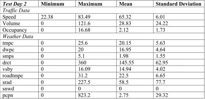
Table 3.4 Statistic summary for test day 2
Test Day 2 Minimum Maximum Mean Standard Deviation
Traffic Data Speed 22.38 83.49 65.32 6.01 Volume 0 121.6 28.83 24.22 Occupancy 0 16.68 2.12 1.73 Weather Data tmpc 0 25.6 20.15 5.63 dwpc 0 20 16.95 4.64 smps 0 5.1 1.98 1.55 drct 0 360 145.55 62.95 vsby 0 16.09 14.94 4.02 roadtmpc 0 31.2 22.5 6.65 srad 0 227.5 58.5 77.7 snwd 0 0 0 0 pcpn 0 823.2 2.75 29.32
Table 3.5 Statistic summary for test day 3
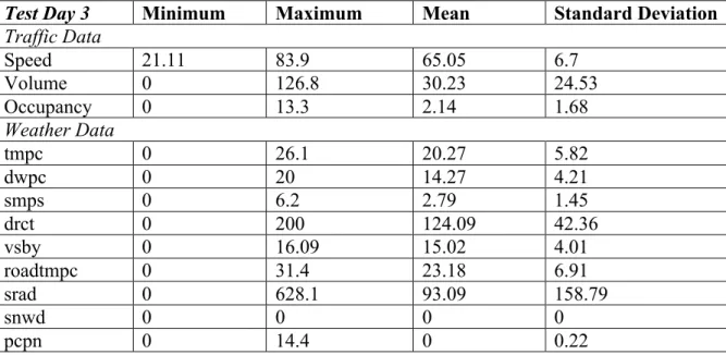
Test Day 3 Minimum Maximum Mean Standard Deviation
Traffic Data Speed 21.11 83.9 65.05 6.7 Volume 0 126.8 30.23 24.53 Occupancy 0 13.3 2.14 1.68 Weather Data tmpc 0 26.1 20.27 5.82 dwpc 0 20 14.27 4.21 smps 0 6.2 2.79 1.45 drct 0 200 124.09 42.36 vsby 0 16.09 15.02 4.01 roadtmpc 0 31.4 23.18 6.91 srad 0 628.1 93.09 158.79 snwd 0 0 0 0 pcpn 0 14.4 0 0.22
CHAPTER 4. LONG-TERM SPEED PREDICTION USING ADVANCED CONVOLUTIONAL NEURAL NETWORK
4.1 Introduction
This chapter discusses the methodology for long-term speed prediction at a route level. Compared to the “short-term” in the next chapter, “long-term” here means “next few hours” or “the next day.”
It has been explained earlier that traffic speed heatmaps of a roadway network over a certain period of time can be viewed as images (see section 1.2). The long-term speed prediction discussed here is predicting the traffic speed image of the next few hours or the next day as the output. Various studies have pointed out that weather is a big impact factor to traffic speeds and traffic incidents have a higher likelihood during adverse weather
conditions. In addition, comparing to future traffic speeds, future weather information is easier to predict and the predicted weather information has been made widely available. Therefore, the predicted weather information will be used as input to predict future traffic speeds. Traffic also follows patterns. The traffic patterns will not change much from week to week on a certain roadway network. Considering that, the historical traffic speeds on the same roadway network should be used as input to predict future traffic speeds as well. Similar to the speed image as output, each piece of the input information can also be
organized spatially and temporally in 2-D matrices and thus be viewed as images. The long-term traffic speed prediction then becomes a problem that needs to convert the image-like inputs to an image-like output. The problem can be formularized as the following.
𝑆𝑝𝑒𝑒𝑑'()*() = 𝑓 𝐼𝑛𝑝𝑢𝑡2, 𝐼𝑛𝑝𝑢𝑡4, … , 𝐼𝑛𝑝𝑢𝑡6 (4.1)
𝑆𝑝𝑒𝑒𝑑'()*() = 𝑠22 𝑠24 𝑠28 𝑠42 𝑠44 𝑠48 𝑠82 𝑠84 𝑠88 ⋯ 𝑠2: 𝑠4: 𝑠8: ⋮ ⋱ ⋮ 𝑠=2 𝑠=4 𝑠=8 ⋯ 𝑠=: 𝑚 = 𝑛𝑢𝑚𝑏𝑒𝑟 𝑜𝑓 𝑙𝑜𝑐𝑎𝑡𝑖𝑜𝑛𝑠 𝑖𝑛 𝑡ℎ𝑒 𝑟𝑜𝑎𝑑𝑤𝑎𝑦 𝑛𝑒𝑡𝑤𝑜𝑟𝑘𝑠 𝑛 = 𝑙𝑒𝑛𝑔𝑡ℎ 𝑜𝑓 𝑡𝑖𝑚𝑒 𝑤𝑖𝑛𝑑𝑜𝑤 𝑡𝑜 𝑝𝑟𝑒𝑑𝑖𝑐𝑡 𝐼𝑛𝑝𝑢𝑡J = 𝑎22 𝑎24 𝑎28 𝑎42 𝑎44 𝑎48 𝑎82 𝑎84 𝑎88 ⋯ 𝑎2:K 𝑎4:K 𝑎8:K ⋮ ⋱ ⋮ 𝑎=K2 𝑎=K4 𝑎=K8 ⋯ 𝑎= K:K , 𝑘 = 1,2, … , 𝐾
In this chapter, a fully convolutional deep network with encoder and decoder is used as the function 𝑓 in the equations above to deal with long-term traffic speed prediction.
4.2 Methodology
To clearly explain the proposed fully convolutional deep network with encoder and decoder used in this chapter, the discussion needs to start from basic ANNs, then talk about the advantage of CNNs, then move to advanced uses of CNN, and finally explain the proposed network in details.
4.2.1 ANN
4.2.1.1 The Basic Building Block
There are many model families in the deep learning world. But no matter whether it is a fully connected network, CNN, or other complicated network such as variational auto-encoder generative adversarial networks (VAE-GAN) (Larsen et al., 2015), they all are rooted from the very basic ANNs. Before the term “artificial neural network” became dominant in today’s modeling field, researchers were all very familiar with the statistical models such as linear regression and logistic regression. Actually, the linear regression model
and logistic regression model can be viewed as ANNs with a single node as well. A single node of ANN is shown as a graph in Figure 4.1.
Figure 4.1 One-node ANN structure As a formula, the output y can be written as:
𝑦 = ℎ 𝑤2𝑥2 + 𝑤4𝑥4 + ⋯ + 𝑤:𝑥:+ 𝑏 (4.2)
or written in matrix format as:
𝑦 = ℎ(𝑊𝑋 + 𝑏) (4.3)
where
𝑊 = 𝑤2 𝑤4 𝑤8 … 𝑤: are the learnable weights
𝑏 is the learnable bias
𝑋a = 𝑥2 𝑥4 𝑥8 … 𝑥
: are the inputs
ℎ is called the activation function 𝑦 is the output
Now, if we recall the formula of linear regression:
𝑦 = 𝑊𝑋 + 𝑏 (4.4)
it can easily be related to ANN and treated as a one node network in ANN context with a special activation function:
Similarly, if we recall the formula of logistic regression:
𝑦 = 2nijk (lmno)ijk (lmno) = 2nijk (p(lmno))2 (4.6) it can be viewed as a one node network in ANN context as well with a well-known sigmoid function as the activation function:
ℎ 𝑥 = 𝑠𝑖𝑔𝑚𝑜𝑖𝑑 𝑥 = 2nijk (pq)2 (4.7)
4.2.1.2 Understand the Capability of ANN
Now both linear regression and logistic regression can be graphically viewed as a one-node ANN shown in Figure 4.1, and the regular ANN is just a stack of lots of connected nodes similar to what is shown in Figure 4.2. Figure 4.2 shows a regular ANN with one output layer and three hidden layers and where each hidden layer has 10 nodes.
Figure 4.2 Fully connected deep ANN
In this typical ANN shown in Figure 4.2, each node functions exactly the same as the signal node case illustrated in Figure 4.1. If this deep ANN structure was used for modeling a problem instead of logistic regression, writing out all the actual formula becomes
To better understand the capability of ANNs, we still use the three-layer ANN shown in Figure 4.2 vs. logistic regression as a comparison. Suppose in both cases we model the same problem and to be specific suppose we have ten inputs (𝑛 = 10), 𝑥2, 𝑥4, … , 𝑥2s, and one output, 𝑦. When modeling the mapping function 𝑓 using logistic regression, we basically use 10×1 = 10 parameters, 𝑤2, 𝑤4, … , 𝑤2s, to capture the dependencies between the inputs and
the output. As a comparison, when using the three-layer ANN shown in Figure 4.2, we use 10×10 + 10×10 + 10×10 + 10×1 = 320 parameters to capture the dynamics. Not only do we use more parameters to model the problem, but also, because of the multiple layers and the nonlinear activation function in each layer, the network can capture higher level nonlinear dynamics than logistic regression can do. In the ANN context, we can easily build a larger and more powerful network by adding more layers or adding more nodes in each layer. In addition, the output is not necessarily restricted to one 𝑦, we can add more nodes in the output layer so that the network can provide multivariate outputs 𝑦2, 𝑦4, … , 𝑦=.
4.2.1.3 How to Train an ANN
An artificial neural network is developed upon very simple building blocks and the theory behind it is that a stack of lots of simple functions can mimic any complex functions. By using simple nonlinear activation functions and multiple layers, the ANN network can model highly nonlinear dynamics. An ANN network is parameterized. Some existing successfully deployed networks contain millions of parameters. Those large networks are extremely powerful, but meanwhile how to find the right values for those millions of
parameters (can also be called weights) is essential and difficult. Ultimately, finding the right values for those millions of parameters in ANN is nothing but an optimization problem and it
is fundamentally exactly the same as finding the weights in a linear regression or a logistic regression.
4.2.1.3.1 Gradient descent
Again, let’s talk about the general method of solving an optimization problem, and then illustrate using linear regression and logistic regression, and finally talk about ANNs. Most of the problems, if not all, can be modeled as optimization problems. For any problem, we always want to achieve some goals. To mathematically and strategically achieve the goal, we need to formularize some objective value regarding our goal and try to minimize or maximize it—this is an optimization problem. An optimization problem can be generally formularized as: 𝑥 = argmin q 𝐽(𝑥) (4.8) where 𝑥 𝑖𝑠 𝑡ℎ𝑒 𝑝𝑎𝑟𝑎𝑚𝑒𝑡𝑒𝑟 𝑤𝑒𝑖𝑔ℎ𝑡𝑠 𝐽 𝑖𝑠 𝑡ℎ𝑒 𝑜𝑏𝑗𝑒𝑐𝑡𝑖𝑣𝑒 𝑓𝑢𝑛𝑐𝑡𝑖𝑜𝑛, 𝑢𝑠𝑢𝑎𝑙𝑙𝑦 𝑖𝑠 𝑎 𝑙𝑜𝑠𝑠 𝑓𝑢𝑛𝑐𝑡𝑖𝑜𝑛
The general method to find the optimal 𝑥 so that the loss function 𝐽(𝑥) can be minimized is gradient descent. Gradient descent comes from a simple and intuitive ideal:
If I can find the direction in which changing 𝑥 increases the value of 𝐽(𝑥), I can change 𝑥 in the opposite direction to make 𝐽(𝑥) smaller. Then I can keep changing 𝑥 in that opposite direction so that 𝐽(𝑥) can be minimized.
The direction “in which changing 𝑥 increase[s] the value of 𝐽(𝑥)” is called gradient, and the method “changing 𝑥 in the opposite direction to make 𝐽(𝑥) smaller” is called gradient descent. Gradient descent is an iteratively updating process and can be generally