Development of multiparametric MRI models for prostate cancer detection based on improved correlative pathology

(1)

Development of Multiparametric MRI Models for Prostate Cancer Detection based on Improved Correlative Pathology

A Dissertation

SUBMITTED TO THE FACULTY OF UNIVERSITY OF MINNESOTA

BY

Chaitanya Kalavagunta

IN PARTIAL FULFILLMENT OF THE REQUIREMENTS FOR THE DEGREE OF

DOCTOR OF PHILOSOPHY

Advisor: Gregory J. Metzger June 2014

(2)

(3)

i

Acknowledgements

This PhD work is based on my original contributions to a large interdisciplinary research project led by Dr. Greg Metzger that involved departmental teams across CMRR, Pathology, Urology, Radiology and Biostatistics.

First of all, I would like to thank my advisor, Greg Metzger, PhD. Greg has been always open to new ideas and has always made himself available to answer my research questions. On a personal level I am grateful to him because I have come this far only because of his support and encouragement.

I would like to thank Drs. Patrick Bolan, Bruce Hammer and Essa Yacoub for being on my thesis committee and for their kind support. I am especially grateful to Prof. Russell Ritenour and Prof. Bruce Gerbi for their guidance towards my academic and career pursuits.

I would like to thank my funding sources NCI RO1 CA131013 (primary funding), NCI R01 CA131013-S1, NIBIB P41 EB015894, UMN Department of Urology Bridge Funding and the UMN Graduate School (Doctoral Dissertation Fellowship)

This project would not have been possible without the support of many people. I am thankful to Drs Xiangmin Zhou (LATIS Image Registration), Joseph Koopmeiners (Predictive Modeling), Stephen Schmechel (Pathology Annotation), and Patrick Bolan (Interpolation and XML parsing scripts).

My thanks to Brian Hanna for his amazing all-round IT support and for being a workplace inspiration. Thanks to Jonathan Henriksen, Laura Moench, Sarah Bowell and Andy Johnson for their help with Pathology processing. Special thanks to Diane Hutter for her help with the blood collection and in scheduling and running the MRI studies. My thanks to our clinical partners Drs

(4)

ii

Badrinath Konety, and Christopher Warlick. Finally, I would like to thank all the people at CMRR who have helped and supported me all these years and made my stay enjoyable.

(5)

iii

Dedication

Jai Sai Ram.

To my parents and my brother who have always encouraged me to achieve new heights.

To my loving daughter Neelu, who is too young to understand the subject matter but is glad that her father is home, my thanks are to you too for cheering me on in your own way.

To my best friend and my wife Janani, there are no words that can express my

(6)

iv

3.1 Synopsis ... 25 3.2 Introduction ... 25 3.3 Methods ... 27 3.3.1 In Vivo MR Data ... 27 3.3.2 Pathology Data ... 28 3.3.3 Image Registration ... 29 3.3.4 Theory ... 31 3.3.5 Multi-Resolution Optimization ... 35 3.3.6 Registration Procedure ... 36 3.3.7 Analysis ... 37 3.3.8 Statistical Analysis ... 38

(8)

vi

3.4 Results ... 39

3.5 Discussion ... 42

3.5.1 Registration Methods ... 42

3.5.2 Registration and Pathology Limitations ... 45

3.5.3 Assessment of Registration Error ... 47

Chapter 4 Developing MP-MRI Cancer Predictive Models using Co-registered regions of Defined Disease ... 49

4.1 Introduction ... 49

4.2 Methods ... 55

4.2.1 Data for Model Development ... 56

4.2.2 Non-cancer from user defined ROIs ... 58

4.2.3 Predictive Modeling ... 59

4.3 Results ... 63

4.4 Discussion ... 70

4.5 Conclusion ... 72

Chapter 5 Application of Methods to High and Ultra High-Field MP-MRI ... 74

5.1 Context ... 74

5.2 Synopsis ... 76

5.3 Introduction ... 76

5.3.1 Theory ... 78

5.4 Methods ... 79

(9)

vii

5.4.2 GaD Solution in AS and OVB Preparation ... 80

5.4.3 Phantom Setup ... 80 5.4.4 MR Instrumentation ... 81 5.4.5 T1 Measurement ... 82 5.4.6 T2* Measurement ... 84 5.5 Results ... 87 5.6 Discussion ... 91

5.6.1 Dependence of R2* on Oxygenation and GaD in Blood... 94

5.6.2 Effect of hyperoxygenation ... 96

5.6.3 Acquisition Methods ... 97

5.7 Conclusion ... 98

Chapter 6 Conclusions ... 100

6.1 Summary and Significance of Findings ... 100

6.1.1 LATIS Image Registration ... 100

6.1.2 MP-MRI Predictive Models ... 101

6.1.3 T1 and T2* Relaxivities of Gd-DTPA in Oxygenated Venous Blood and Aqueous Solution at 3 and 7T. ... 103

6.2 Future Work ... 104

6.2.1 Correlation of MRI with Quantitative Pathology ... 104

6.2.2 Variation of the L5P_CGROI Model ... 105

(10)

viii

List of Tables

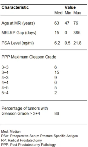
Table 2.1 Patient Population Clinical Characteristics ... 9 Table 2.2 MP-MRI study acquisition parameters... 11 Table 3.1 Multi–user registration accuracy metric statistics ... 42 Table 4.1 A comparison of visual assessment and predictive model resultant combinations of MP-MRI datasets in the prediction of PCa. ... 53 Table 4.2 Characteristics of data pool (number, name, origin and type of cancer and non-cancer data) used in model generation. ... 59 Table 4.3 Classification accuracy summaries for various modeling approaches used to develop a MP-MRI model for predicting PCa using cancer and non-cancer data in the peripheral zone only (Data Pool I). The LASSO 5 parameter approach was chosen based on these results. ... 61 Table 4.4 Total number of cancer and non-cancer voxels from each data pool used for Single Predictor (SP) and Multi Predictor (MP) model generation. The difference in the number of initial and final cancer and non-cancer MP voxels in CG, ALL and CGROI pools is due to a sampling cutoff of 200 voxels from each

region used in the R code for faster processing. A comparison of the results obtained using all voxels with those obtained using a 200 voxels cutoff showed no difference. ... 63 Table 4.5 Median, 95% confidence intervals for qMR cancer and non-cancer values from data pools used in 5 parameter model generation. Also shown are the p values showing whether cancer qMR values are statistically significant from non-cancer values. ... 64 Table 5.1 Acquisition parameters for R2* calculations. ... 86

(11)

ix

Table 5.2 R1 and R2* values for Oxygenated Venous Blood (OVB) and Aqueous

Solution (AS) at 3T and 7T at 37 ºC. ... 88 Table 5.3 T1 relaxivities (r1) of Gd-DTPA in Oxygenated Venous Blood (OVB)

and Aqueous Solution (AS) at 37 ºC for both 3 and 7T along with respective pO2,

sO2 and Hematocrit (Hct) ranges used for the measurements. ... 88

Table 5.4 Relationship of Gd-DTPA concentration [GaD] with R2* in Aqueous Solution (AS) and Oxygenated Venous Blood (OVB) at 3T and 7T. ... 89 Table 5.5 A review of T1 relaxivities (r1) of Gd-DTPA (GaD) in water published in

literature. ... 92 Table 5.6 A review of T1 relaxivities (r1) of Gd-DTPA (GaD) in blood published in literature. ... 93

(12)

x

List of Figures

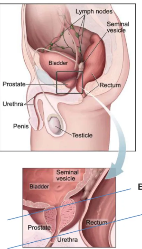
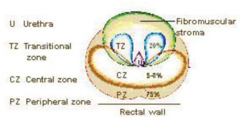
Figure 1.1 shows the anatomy of the prostate in relation to other pelvic structures. Inset figure shows an enlarged view along with the base and apex. This image is provided courtesy of the National Cancer Institute website (http://www.cancer.gov). ... 2 Figure 1.2 shows an axial view of the prostate showing zonal anatomy. The central gland (CG) as defined in this thesis (not shown in figure) is composed of everything other than PZ (i.e. TZ, CZ, Fibromuscular stroma). This image has been provided courtesy of SEER Prostate Cancer Training Module, U.S. National Institutes of Health, National Cancer Institute (http://training.seer.cancer.gov/). .. 3 Figure 1.3 shows the zonal anatomy of the prostate as seen on a T2-weighted

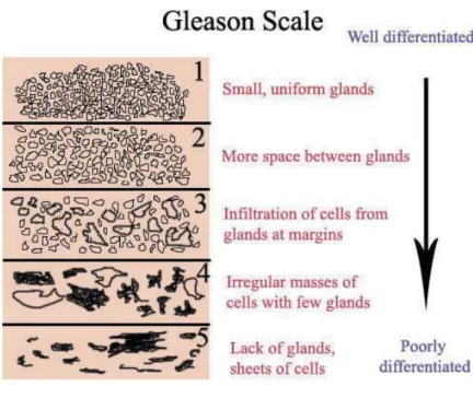
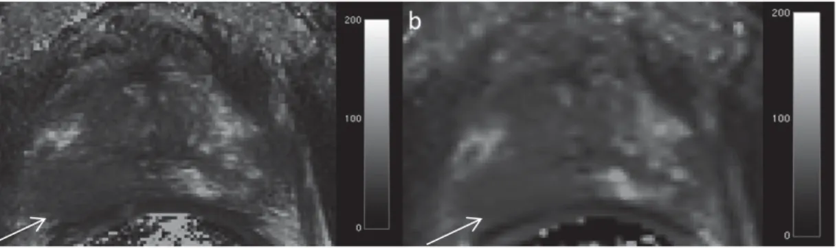
MRI. The axial (a) and sagittal (b) images were obtained on a 3T Siemens Magnet using an endorectal coil (ERC). The center of the urethra is depicted by the yellow line. ... 3 Figure 1.4 Gleason Scale (image courtesy – Wikimedia.org). ... 5 Figure 2.1 T2-weighted image of the prostate. Hypointense region (arrow)

indicates cancer. The units of the scale bar are in ms. ... 12 Figure 2.2 T2-maps of the prostate using (a) T2-TSE (Turbo Spin Echo) (b) T2

-SEMC (Spin Echo Multi Contrast) methods. Hypointense region (arrow) indicates area of cancer. The units of the scale bars are in ms. ... 13 Figure 2.3 (a) T1-weighted image and T1 map (DESPOT1) (54) of the prostate.

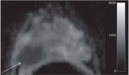
The units of the scale bars in are SI units (a) and ms (b). ... 15 Figure 2.4 Apparent Diffusion Coefficient (ADC) map of the prostate. This image was obtained with a diffusion weights (b) of 50, 400 and 800 s/mm2. Hypointense

(13)

xi

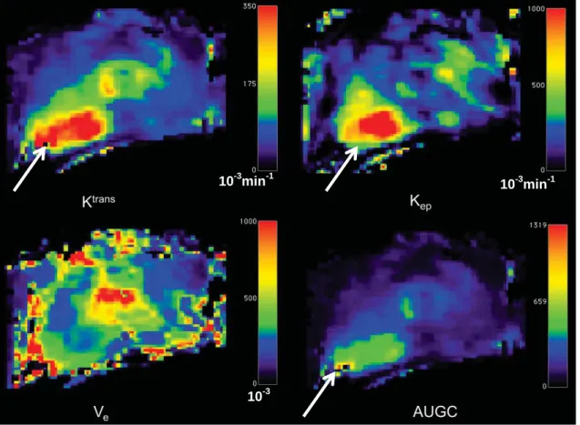
region (arrow) is indicative of restricted diffusion (cancer). Units of scale bar are in 10-6 mm2s-1. ... 16 Figure 2.5 DCE-MRI maps of the prostate. Units of the scale bar are 10-3 × min-1 (Ktrans), 10-3 × min-1(Kep) and 10-3 (Ve). Increased Ktrans (wash-in), Kep (wash-out)

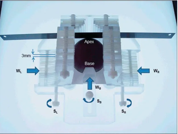
and AUGC (Area Under Gadolinium Concentration Curve) identifies area of cancer in these maps. ... 19 Figure 2.6 Prostate sectioning box made of Acrylic and Teflon. The box is shown with a spherical prostate model and the movable walls on the left (WL) right (WR) and base (WB) are pushed in to hold the model securely. Each moveable wall is held in place with a locking screws SL, SR and SB, respectively. A standard pathology blade is inserted through the milled slits in the acrylic pieces that make up the left and right walls. Each successive axial cut through the prostate requires passing through the next slit in the side walls. The tolerance is such that the blade can only traverse through the corresponding slit on the opposite side. ... 21 Figure 2.7 Diagrams of pathologic sectioning protocol overlaid on a coronal (a) and axial (b) T2w image. After placing the prostate in the sectioning box, the first

cut made is approximately 0.6 mm from the apex of the gland to create the apical section, with successive axial cuts 3mm apart moving towards the base. The axial cross-sections are designated by letters “A”, “B”, “C”, etc., depending on the size of the prostate, with “A” being the most apical slice. Slices are divided into four quarters (b). Each quarter is labeled based on the letter of the slice from which it comes and its position in the slice (e.g. anterior/posterior = A/P and right/left = R/L). After removal from the box, the apical portion is sectioned in 2mm intervals with parallel cuts emanating from the urethra. The sections near

the urethra are labeled “RDUMA” (right distal urethral margin A) and “LDUMA”

(14)

xii

labeled “RDUMB” and “LDUMB”, etc. This process continues out to the lateral

margins of the apical section. Each slice section is then embedded in a paraffin block and one 4-micrometer H&E-stained slide is prepared from each section and digitized. A pathologist then digitally annotates the prostate capsule (red contour) and cancer regions (brown contour) on each slide. ... 22 Figure 2.8 (a) Slides from a complete axial slice are then manually assembled into a PWM by aligning the capsule annotations of the quartered pathology sections to form a continuous capsule while minimizing the overlap of tissues between the combined sections (b). ... 23 Figure 3.1 A schematic demonstrating the procedure to co-register pathology to T2w MRI using LATIS. First, the source (a) and target (b) images are segmented,

scaled and translated. Second, the prostate capsule and internal structure masks are identified to constrain the pathology transformation. The source and target masks (d and e) are registered and a transformation matrix is obtained. Images (c) and (d) show the transformation flow matrix and applied deformation field respectively. Third, the transformation matrix is applied (red arrow) to the pathology (f) which places it in spatial correspondence to the T2w MRI resulting in

(g).Lastly, applying the transformation matrix to each one of the annotated cancer regions (i) places them in the spatial framework of the anatomic T2w

images (j). ... 28 Figure 3.2 Registration results. Column ‘a’ shows the masked PWM with

annotated tumor regions. Column ‘b’ shows the registered tumor regions overlaid

on the ERCinMR. Column ‘c’ shows the original ERCinMR. ... 40 Figure 3.3 Registration accuracy metric calculation workflow - (a) Feature marked masked PWM. (b) Corresponding features on ERCinMR. (c) Warped feature embedded masked PWM. (d) Feature embedded masked ERCinMR. .. 41 Figure 4.1 Process of acquiring data for predictive model generation. ... 55

(15)

xiii

Figure 4.2 Visualization of cancer and non-cancer regions used in model generation from four patients on the un-interpolated T2w anatomic images. PCa is confined to (a) CG only (b) PZ only (c) both CG and PZ. (d) shows an example of a non-cancer user defined ROI in the CG (NCCG-ROI). PC stands for

Pseudo Capsule. The CG (green) and PZ (yellow) annotations provided the original segmentation of the two prostatic regions. These annotations are mostly overlapped by the other annotation therefore they only appear as broken curves in this figure. ... 58 Figure 4.3 L5P_PZ model results. (a) ROC curve for L5P model and ADC showing the ROC0.1 cutoff (b) Table showing AUC and ROC0.1 values for each

single predictor and L5P_PZ model. L5P_PZ results are shown in order of incremental addition of significant predictor to the model. Plots (c) and (d) show

the L5P_PZ model’s performance for cancer and non-cancer regions of different size by the calculation of sensitivity per cancer region and specificity per non cancer region. ... 65 Figure 4.4 L4P_CG model results. (a) ROC curve for L4P_CG model and ADC showing the ROC0.1 cutoff (b) Table showing AUC and ROC0.1 values for each

single predictor and L4P_CG model. L4P_CG results are shown in order of incremental addition of significant predictor to the model. Plots (c) and (d) show the L4P_CG model’s performance for cancer and non-cancer regions of different size by the calculation of sensitivity per cancer region and specificity per non cancer region. ... 66 Figure 4.5 L4P_ALL model results. (a) ROC curve for L4P_ALL model and ADC showing the ROC0.1 cutoff (b) Table showing AUC and ROC0.1 values for each

single predictor and L4P_ALL model. L4P_ALL results are shown in order of incremental addition of significant predictor to the model. Plots (c) and (d) show

(16)

xiv

size by the calculation of sensitivity per cancer region and specificity per non cancer region. ... 67 Figure 4.6 L5P_CGROI model results. (a) ROC curve for L5P_CGROI model and

ADC showing the ROC0.1 cutoff (b) Table showing AUC and ROC0.1 values for

each single predictor and L5P_CGROI model. L5P_CGROI results are shown in

order of incremental addition of significant predictor to the model. Plots (c) and (d) show the L5P_CGROI model’s performance for cancer and non-cancer regions

of different size by the calculation of sensitivity per cancer region and specificity per non cancer region. ... 68 Figure 4.7 72 year old man with biopsy-confirmed PCa with Gleason score, 6 on the right side PZ of the prostate. (a): PWM with tumor outlined in blue. (b)Corresponding T2-weighted MRI with registered tumor region overlay, and (c)

composite biomarker score (CBS) map acquired using a L5P_PZ model with registered tumor region outline in black. Associated CBS colorbar shows ROC0.1 cutoff. The PZ tumor region can be seen appreciated in against the background in the CBS map and is composed of pixels with CBS > cutoff. ... 69 Figure 5.1 (a) Axial and (b) sagittal scout images of the phantom setup. Legend: 1, water bath tubing; 2, outer plastic container; 3, 0.45% saline water; 4, vial; 5, vial holder; 6, inner plastic container. Coronal view of the oxygenated venous blood (OVB) phantom from the first echo of the multi-echo acquisition used for calculating R2* for (c) 3 T and (d) 7 T. Coronal view of the OVB phantom from the

TI = 20 ms, inversion recovery- turbo flash (IR-TFL) acquisition for (e) 3 T and (f)

7 T. The location of circular regions of interest used for data analysis within each

acquisition for the zero GaD vial are shown in (c)–(f). ... 82 Figure 5.2 Plots of R1 and R2* vs [GaD] for oxygenated venous blood (OVB) and

aqueous solution (AS) at 3 and 7 T. Plots of relaxivity modeled with linear (red)

(17)

xv

R1 relaxivity (r1) for 3 and 7 T in both AS (a, b) and OVB (c, d). A linear model

was also used to calculate R2* relaxivity (r2*) in AS (e, f). To determine r2* in

OVB, a quadratic function for [GaD] ≤ 2 mM and linear function for [GaD] ≥ 2 mM

was found to characterize the data better than a quadratic fit alone over the whole range of [GaD] (g, h). ... 90

(18)

xvi

List of Abbreviations

PCa – Prostate Cancer

MRI – Magnetic Resonance Imaging MP-MRI – Multiparametric MRI DWI – Diffusion Weighted Imaging DCE – Dynamic Contrast Enhanced

MRSI – Magnetic Resonance Spectroscopy Imaging ADC – Apparent Diffusion Coefficient

CG – Central Gland PZ – Peripheral Zone TZ – Transition Zone CZ – Central Zone

PSA – Prostate Specific Antigen DRE – Digital Rectal Exam

TRUS – Transurethral Ultrasound GS – Gleason Score

qMR – Quantitative MR ROI – Region of Interest

GFR – Glomerular Filtration Rate RP – Radical Prostatectomy ERC – Endorectal Coil T2w – T2 weighted TSE – Turbo Spin Echo

SEMC – Spin Echo Multi Contrast EPI – Echo Planar Imaging

(19)

xvii

DESPOT1 – Driven Equilibrium Single Pulse Observation of T1 VIBE – Volume Interpolated Breathold Examination

SAR – Specific Absorption Rate TE – Echo Time

Ktrans– Forward Volume Transfer Constant

Kep– Reflux Rate between the Extracellular Space and the Plasma

Ve– Fractional Extravascular Extracellular Space

AUGC – Area Under Gadolinium Curve AIF – Arterial Input Function

H&E – Hematoxylin and Eosin PWM – Pseudo Whole Mount

QMHS – Quarter Mount Histological Section

LATIS – Local Affine Transformation guided by Internal Structures DSC – Dice Similarity Coefficient

ERCinMR– in vivo MR image obtained using ERC TRE – Target Registration Error

inMR – in vivo MR exMR – ex vivo MR MI – Mutual Information

COFEMI – COmbined Feature Ensemble Mutual Information SWMI – Spatially Weighted Mutual Information

BSp – Beta Spline TPS – Thin Plate Spline

ANN – Artificial Neural Network

GEE – Generalized Estimating Equations CAD – Computer Aided Diagnosis

(20)

xviii IL – Index Lesion

SL – Secondary Lesion IL – Tertiary Lesion PC – Pseudo Capsule

ROC – Receiver Operator Characteristic

ROC0.1– Sensitivity value on ROC curve corresponding to 90% specificity

CBS – Composite Biomarker Score

LASSO – Least Absolute Shrinkage and Selection Operator OVB – Oxygenated Venous Blood

CA –Contrast Agent AS – Aqueous Solution GaD – Gd-DTPA

IR-TFL – Inversion recovery Turbo Flash pO2– Partial Pressure of O2

sO2– Hemoglobin Oxygen Saturation

Hct – Hematocrit

T1– Longitudinal Relaxation Time

T2– Transverse Relaxation Time

T2* – Apparent Transverse Relaxation Time

R1– Longitudinal Relaxation Rate

R2– Transverse Relaxation Rate

R2* – Apparent Transverse Relaxation Rate

r1– T1 relaxivity

(21)

xix

Thesis Statement

Prostate cancer (PCa) is a prevalent disease which affects 1 in 6 men in the United States and has overtaken lung cancer as the leading cause of cancer related deaths in American men and number two worldwide (1). While diagnosis and treatment options are improving, there is still a fundamental problem with its management. It is unclear which PCa is aggressive (life- threatening) and which is non-aggressive (non-life threatening). As a result, overtreatment of PCa results from the absence of tools that can properly differentiate between the two. While magnetic resonance imaging has become an increasingly valuable tool in the management of men with PCa, its use to identify aggressive disease and characterize extent have yet to be developed. The ability to identify the extent of significant disease would increase the effectiveness of focal therapy including cryosurgery and RF ablation which are currently hampered by the absence of good information for targeting treatment. Currently available treatments such as radiation therapy and surgery address the whole gland, while focal therapies treat part of the gland and can more effectively avoid damaging critical structures. Improved detection and evaluation of extent will impact areas of prostate cancer management by improving biopsy yield especially with the growth of MRI targeted biopsies both in the gantry and fused with real-time Ultrasound(2).

Among several diagnostic imaging tests that are available for detection of PCa in the market today, Magnetic Resonance Imaging (MRI) occupies a unique position due to its excellent soft tissue contrast and its ability to generate tissue property dependent multi-parametric data (3). Multi-parametric MRI (MP-MRI) refers to the combination of multiple imaging methods and their associated

(22)

xx

quantitative maps such as apparent diffusion coefficient (ADC) maps from diffusion weighted imaging (DWI), pharmacokinetic maps from dynamic contrast enhanced MRI (DCE-MRI) and metabolite ratio maps from three dimensional MR spectroscopic imaging (3D-MRSI). With DWI, MP-MRI can help in tumor identification by mapping areas of restricted diffusion of water molecules that indicate micro-structural changes in cellular density. Angiogenesis, the growth of new blood vessels, is an indicator of cancerous tissue. Using DCE-MRI, we can probe heterogeneous neovascular structure and abnormal vessel permeability that is indicative of cancer. 3D-MRSI is another MR technique that detects cancer by mapping the chemical composition of the prostate (2,3). MP-MRI has been shown to increase sensitivity and specificity compared to any single MRI dataset.

The ability to develop and evaluate MP-MRI to prospectively detect disease, assess aggressiveness and delineate extent, first requires the retrospective validation against post-surgical pathology sections. Despite the large effort made by many groups in this area of research, the correlation of in vivo MP-MRI with pathology is still a challenge and to date is insufficient to develop highly accurate models of disease. To address this problem this thesis showcases:

1. A novel registration approach called LATIS (Local Affine Transformation assisted by Internal Structures) for co-registering post prostatectomy pseudo-whole mount (PWM) pathological sections with in vivo MRI images. This work is presented in Chapter 3.

2. A MP-MRI based predictive model for disease detection using a composite biomarker score based on a unique database of pathology co-registered MR data sets. This work is presented in Chapter 4.

(23)

xxi

Chapter 2 details the clinical characteristics of the patient cohort and the MP-MRI acquisition methods and post processing used to generate the data used in chapters 3 and 4. Chapter 5 reports on a study where the r1 and r2* relaxivities of

a common paramagnetic contrast agent are measured in blood and saline at both 3T and 7T. This is important information to have when attempting to perform DCE-MRI studies as part of a MP-MRI protocol. Previous studies done by Metzger et al. (4) have shown that, R2* effects of typical paramagnetic

contrast agents make the determination of subject dependent arterial input functions impossible at 7T and results in an underestimation of pharmacokinetic parameters even if a model based function is used. Similar effects are expected to negatively impact other contrast enhanced studies when performed at 7T such as first pass perfusion and angiography exams relying on T1-weighted enhancement (5). Finally, Chapter 6 reports on some initial studies comparing MP-MRI with quantitative pathology while also highlighting future directions for the work contained in this thesis.

(24)

1

Chapter 1

Introduction

1.1 Prostate Cancer

According to the GLOBOCAN (Global Burden of Cancer Study) project, which provides contemporary estimates of the incidence, mortality and prevalence from major types of cancer at the national level, for 184 countries of the world, Prostate Cancer (PCa) was the second most common cancer among men worldwide (1) as of 2012. It is estimated that in 2014, 233,000 new cases of PCa will be diagnosed and 29,480 men will die of this disease in the United States alone(6). According to the American Cancer Society, 98.9% of men survive for five years or more after being diagnosed with all stages of PCa (local, regional or distant) (6). The increase of this 5-year survival percentage from 98.9 to 100% for men diagnosed with localized and regional PCa is attributed to early diagnosis of disease (7).

1.2 Prostate Anatomy

The prostate is a walnut-sized gland (Figure 1.1) located inferior to the bladder, superior to the penis and anterior to the rectum. A healthy prostate weighs around 20 to 25 grams, has a volume around 20 cc and measures around 3 cm x 4cm x 2cm. The prostate consists of a base, an apex, anterior, posterior and two lateral surfaces and has the urine in the bladder run through its center via the urethra. The main function of the prostate is to produce a thin, milky fluid containing citric acid and acid phosphatase that is added to the seminal fluid at the time of ejaculation. Also seen in Figure 1.1 are the seminal vesicles, which are a pair of small tubular glands that are attached to the vas deferens (carrying-away vessels) at the base of the bladder. The seminal vesicles produce fructose

(25)

2

that helps with the sperm motility. The fluid from the seminal vesicles makes up most of the volume of the ejaculatory fluid (8-13).

Figure 1.1 shows the anatomy of the prostate in relation to other pelvic structures. Inset figure shows an enlarged view along with the base and apex. This image is provided courtesy of the National Cancer Institute website (http://www.cancer.gov).

The prostate gland is divided into three distinct glandular regions each distinguishable from the other on the basis of histology, anatomical landmarks and susceptibility to pathologic disorders (14). These are the peripheral zone (PZ), which covers 70% of the prostate, central zone (25%), transition zone (TZ) (5%) and anterior Fibromuscular Stroma (5%). Figures 1.2 and 1.3 show these glandular zones in the form of a diagram and as seen on a T2-weighted MRI

image respectively.

Base

(26)

3

Figure 1.2 shows an axial view of the prostate showing zonal anatomy. The central gland (CG) as defined in this thesis (not shown in figure) is composed of everything other than PZ (i.e. TZ, CZ, Fibromuscular stroma). This image has been provided courtesy of SEER Prostate Cancer Training Module, U.S. National Institutes of Health, National Cancer Institute (http://training.seer.cancer.gov/).

Figure 1.3 shows the zonal anatomy of the prostate as seen on a T2-weighted MRI. The

axial (a) and sagittal (b) images were obtained on a 3T Siemens Magnet using an endorectal coil (ERC). The center of the urethra is depicted by the yellow line.

ERC

ERC Bladder

L R

(27)

4

1.3 Cancer Diagnosis

Adenocarcinomas (cancerous tumors) that arise from the glandular tissue make up 95% of PCa tumors. 75% of all PCa arises in the PZ, 20% in the TZ and about 5-10% in the CZ while local extension of disease tends to be into capsule, bladder base and the seminal vesicles. PCa usually does not present any symptoms unless it reaches a very advanced stage. Most common local symptoms present themselves are urinary outflow obstruction and back pain (15). The serum PSA (Prostate Specific Antigen) level test, DRE (Digital Rectum Examination) and TRUS (Transrectal Ultrasound) guided biopsy are the three clinical examinations used for early diagnosis of PCa. A prostate biopsy is recommended to patients with an elevated PSA level (> 4 ng/mL) in their blood and a suspicious induration on DRE. TRUS guided biopsy is the current gold-standard for prostate biopsies. While a prostate biopsy may be performed to confirm the presence of tumor at the location of a positive DRE and detect the cause of the elevated PSA, TRUS guided biopsies have shown low sensitivity (23-42%) (16,17).

Biopsy results are graded with a Gleason Score (GS) which is based on the glandular pattern description of the tumor. The GS is a two part sum of the primary (predominant) and secondary (second most prevalent) grades, each on a scale of 1 (well differentiated) to 5 (least differentiated). Well-differentiated cancer cells resemble normal cells and are inclined to grow and spread at a slower rate than un-differentiated cancer cells that may lack normal tissue architecture (Figure 1.4). The GS score ranges from 2 to 10 and indicates the likeliness of a tumor to spread. A GS of 7 (3+4 or 4+3) is considered clinically significant with a worse prognosis than a GS of 6 (i.e. 3+3) (18-22).

(28)

5

Figure 1.4 Gleason Scale(image courtesy – Wikimedia.org).

1.4 Multiparametric MRI in the detection of

Prostate Cancer

Among several diagnostic imaging modalities that are available for detection of PCa, Magnetic Resonance Imaging (MRI) occupies a unique position due to its excellent soft tissue contrast and its ability to generate tissue property dependent multi-parametric data (3). Conventional imaging techniques like CT have found limited use in PCa detection because of insufficient spatial and contrast resolution (23-25). PET/CT is currently used for detection of post-treatment recurrence and has not shown conclusive detection capabilities for primary PCa diagnosis (26-28). MP-MRI is currently one of the most promising tools for PCa detection and staging with the potential to further impact disease management by characterizing disease aggressiveness and extent (12,29-34). MP-MRI refers to

(29)

6

the combination of multiple imaging methods and their associated quantitative maps such as T2 maps associated with T2-weighted imaging, ADC maps from

diffusion weighted imaging (DWI), pharmacokinetic maps from dynamic contrast enhanced MRI (DCE-MRI) and metabolite ratio maps from three dimensional MR spectroscopic imaging (3D-MRSI). Quantitative MRI (qMR) parameters like T2,

ADC, Ktrans, Kep, Ve, AUGC and those derived from MRS (Magnetic Resonance

Spectroscopy) acquisitions have been shown to detect PCa and correlate with tumor grade (35-38). MP-MRI guided biopsy has shown good results in detecting significant disease and could reduce unnecessary biopsies (39,40).

1.5 Multiparametric MRI based Predictive Models

in the Detection of Prostate Cancer

The ground truth in PCa detection is given by pathology. One way to achieve pathology comparable detection using MP-MRI is by the construction of a model that accurately predicts disease as defined on pathology. An MP-MRI model provides a standardized approach of combining multiple datasets for maximizing the predictive power of MP-MRI. A vast body of literature exists in the prediction of PCa using MP-MRI models and there are new studies being added every day (18-24). The process of assessing MP-MRI’s ability to predict what is currently only obtained through post prostatectomy pathology (PPP), involves correlating MP-MRI obtained in-vivo (inMR) with post-surgical specimens. This correlation with the pathologic Gold Standard involves the transfer of information obtained from pathology (i.e. grade and location of identified disease). This mapping has been accomplished through a variety of methods in the literature: manual mapping of regions of interest (ROIs) (41); visual mapping of sextants (42) or octants (43,44); mapping locations of graded MR guided biopsy specimens (45) or calculated Gleason scores (43,46,47). The process of correlating manually

(30)

7

drawn regions of interest (ROIs) (41) on the MRI corresponding to identified areas of disease on pathology introduces potential biases of ROI drawing and placement used to generate predictive models. On the other hand using pathologically correlated slice sections (sextants (42), octants (43,44)) on MP-MRI is prone to data averaging when a section contains a mix of cancer and non-cancer tissue. These issues are addressed in this thesis (Chapter 4) where global anatomic features are used to guide a deformable registration method (LATIS) which is then used to map pathologist annotated regions of cancer directly to endorectal coil obtained in-vivo MRI images (48). The location size and extent are defined by global anatomic features. While an assumption is made about coincident slice locations and there is user interaction involved in defining internal structures for guiding the deformable registration methods, these are arguably less biased than other proposed methods. This image registration method is used to generate co-registered datasets which are then used in the development of MP-MRI based predictive models for the detection of PCa (Chapter 4).

(31)

8

Chapter 2

Materials and Methods

2.1 Patient Population

The patient cohort used in this thesis consisted of those who had biopsy confirmed PCa and were scheduled to undergo prostatectomy (46 men, age range 47 to 76 years with a median age of 63 years). All patients underwent imaging at the Center of Magnetic Resonance Research between November 2009 and August 2012 after biopsy and before surgery after providing written consent under an Institutional Review Board approved protocol. The exclusion criteria included contraindications to endorectal coil placement including severe hemorrhoids, latex allergy, surgically absent rectum, severe inflammatory bowel disease; contraindications for MRI including ferromagnetic implants, history to

shrapnel or shot gun injury, body mass index ≥ 40, cardiac pacemakers,

claustrophobia, large tattoos, hip replacement and penile implants; contraindications to contrast agents including strong history of asthma and allergies, colostomy, kidney disease and Glomerular Filtration Rate (GFR) < 30 ml/min and prior treatment or procedures to treat PCa. Men received radical prostatectomy (RP) after an average gap of 27 days post MRI (range: 0-385 days). The maximum gap of 385 days corresponds to a patient who was initially on active surveillance but underwent RP later. Quarter mounted histopathological sections were generated from the surgical prostate specimens. Table 2.1 shows the clinical characteristics summary of the patient population.

(32)

9

Table 2.1 Patient Population Clinical Characteristics

2.2 MRI acquisition and Parametric Mapping

2.2.1 Imaging Setup

Patients were imaged on a 3T scanner (Siemens Healthcare, Erlangen Germany) transmitting with the whole body coil and receiving with a balloon-type endorectal coil (ERC) combined with an external surface array. The surface array consisted of two rows of 3 elements anteriorly from a flexible body coil and two rows of 3 elements posteriorly from a spine coil. The ERC was inserted after the patient assumed the left lateral decubitus position and inflated with 60 ml of

(33)

10

perfluorocarbon to reduce air induced susceptibility artifacts. Rotating back into the supine position, the anterior surface array was positioned with the coil centered at the level of the greater trochanter in the foot-head direction. In later studies, a urethral catheter (Bard, Latex radiopaque urethral catheter, Robinson model, 18Ch/ french-6.0mm) was inserted with the ERC to provide a pathway to release gas from the rectum which otherwise would build up behind the endorectal coil. While not explicitly quantified, the use of the urethral catheter appeared to relieve the issue of gas in the bowel. In addition, it was inexpensive and did not affect study workflow or patient comfort as an endorectal coil was already being inserted. Other than instructing subjects to be nil per os (ingesting no fluids or solids) 4 hours prior to the study, no additional anti-peristaltic or preparation measures were taken.

2.2.2 MRI Acquisitions Overview

Scout images of the prostate in the sagittal, axial and coronal planes were acquired initially to check the depth and rotation of the ERC. After confirming the adequate positioning of the ERC, the rest of the MRI study proceeded and included the following acquisitions.

1. Anatomic imaging using a T2-weighted (T2w) Turbo Spin Echo (T2-TSE)

sequence in the axial, sagittal and coronal planes.

2. Additional TSE datasets acquired in the axial plane at different echo times for calculating T2 maps (T2-TSE).

3. T1-weighted Turbo Spin Echo (T1-TSE) imaging for the detection of

post-biopsy hemorrhage.

4. Multi Echo Spin Echo imaging as an alternative method for calculating T2 maps (T2-SEMC).

5. Single Shot Echo Planar Imaging (EPI) diffusion weighted imaging (DWI) for calculation of Apparent Diffusion Coefficient (ADC) maps.

(34)

11

6. 3D gradient echo data sets for calculating T1 maps using DESPOT1 (Driven

Equilibrium Single Pulse Observation of T1).

7. Dynamic Contrast Enhanced MRI (DCE-MRI) using 3D Flash VIBE (Volume Interpolated Breathold Examination (T1w3D-GRE).

Acquisition parameters are tabulated in Table 2.2. All studies were run in the first-level control mode with prostate specific power and B0 adjustment. Further

details for each acquisition and the calculation of parametric maps used for subsequent modeling are detailed below.

(35)

12

2.2.3 T

2

w Anatomic imaging

Figure 2.1 T2-weighted image of the prostate. Hypointense region (arrow) indicates

cancer. The units of the scale bar are in ms.

T2-weighted (T2w) MRI is the traditional method of imaging the prostate and

determining the location of PCa. On T2w sequences, in general, normal prostate

PZ areas show high signal intensity owing to high water content whereas the CG areas (comprising of central and transition zones) show lower signal intensities. While PCa is frequently seen as a hypointense region in the PZ, some cancers are isointense and therefore cannot be seen on T2w images. T2w sequences

show low specificity due to the high frequency of low intensity regions due to prostatitis, atrophy and calcifications (32). Hypointense regions can also be seen with areas of hemorrhage (post-biopsy or otherwise) infection and as a result of radiation or hormonal treatment. For this reason a gap of at least six to eight weeks post-biopsy is suggested prior to performing MRI.

After confirming accurate endorectal coil placement, anatomic images were acquired using a T2-weighted (T2w) fast spin echo or Turbo Spin Echo (T2

(36)

13

acquired with a left-right phase encoding and no parallel imaging acceleration. In cases where the predicted specific absorption rate (SAR) was too high, the repetition time (TR) of the transverse scan was increased accordingly resulting in a nominal repetition time of 6 s. All axial images were positioned such that the slice plane passed perpendicular to the posterior surface of the prostate. Coronal and sagittal T2w-TSE anatomic scans were acquired in orthogonal planes with

respect to the transverse acquisitions with a TE of 107 ms and an acceleration factor of 2 with right-left and foot-head phase encoding directions, respectively. No SAR issues were present in these other orientations as fewer slices were acquired.

2.2.4 T

2

mapping

Figure 2.2 T2-maps of the prostate using (a) T2-TSE (Turbo Spin Echo) (b) T2-SEMC

(Spin Echo Multi Contrast) methods. Hypointense region (arrow) indicates area of cancer. The units of the scale bars are in ms.

While T2w anatomic imaging provides the best anatomic detail of the prostate’s

zonal anatomy and margins, there is evidence that there may be an advantage to calculating T2 maps (49,50). T2 mapping provides a measure of the apparent

transverse relaxation time in milliseconds (ms) on a voxel by voxel basis. Measuring relaxation times instead of relying of image intensities as in T2w

(37)

14

imaging, is an ideal way to parameterize the anatomic images. The potential advantages result from the ability to use an absolute value for differentiating tissue and observing therapeutic effect. When there is little normal tissue within a given image it becomes difficult to interpret abnormal regions based solely on signal intensity. Figure 2.2 shows two ways of achieving T2-maps of the prostate

used in this research.

The first method involved acquiring additional axial TSE data sets with echo times of 30, 74 and 144 ms. To accelerate acquisitions of these additional series, parallel imaging with an acceleration factor of 2 was used resulting in a scan time of 2:28s per series. The mapping of T2 from these data was

accomplished by methods previously described and validated by Liney et al. (51) and Gibbs et al.(52). Transverse relaxation rates were calculated through a semi-logarithmic linear least squares fit to the signal intensity equation,

S = S₀e-TET₂

(2.1) where S0 represents the signal at TE=0 ms (the proton density signal) and S is

the signal intensity at a given TE from the multiple TSE datasets acquired at different echo times. The function LINFIT in IDL (ITT Boulder, CO) was used to compute this value. The T2-TSE mapping approach was chosen due to its

acquisition and hence anatomical similarity to the T2-weighted acquisition. This is

especially important during the transfer of pathology registered tumor regions from the T2-weighted image to the T2 map. The T2-TSE approach is also more

time-efficient compared to the multiecho approach and as a result is less prone to motion artifacts.

As an alternative to the T2 maps generated by the multiple TSE

acquisitions described above, a spin echo multi-contrast (SEMC) acquisition was also obtained. In this type of sequence, the echoes of the spin echo train each contribute to a different image with varying T2-weighting. A total of 11 echoes

(38)

15

154.1 ms. The disadvantage of this acquisition compared to the multiple TSE imaging series for generating T2 maps was a decrease in resolution and increase

in scan time while the advantage was the freedom from motion artifacts between images of each echo time and the availability of more datasets for T2

quantification. Because of the presence of more points along the T2 decay curve,

a non-linear fit using the function CURVEFIT in IDL was used. It was important to remove the image generated from the first echo of the series as this first point exhibited non-monoexponential characteristics. The signal of the first point is a pure echo whereas signals acquired at subsequent TEs are composed of primary and stimulated echoes as the refocusing pulse flip angles are not exactly 180˚ due to B1 field inhomogeneities. This first point was not included as it would have

led to an overestimation of T2 (53).

2.2.5 T

1

-weighted imaging and mapping

Figure 2.3 (a) T1-weighted image and T1 map (DESPOT1) (54) of the prostate. The units

of the scale bars in are SI units (a) and ms (b).

In this work, a T1-weighted Turbo Spin Echo (T1-TSE) sequence was used

for the qualitative assessment of post-biopsy hemorrhage. While an effective means to avoid misreading the associated T2-weighted images, the use of the qualitative T1-weighted images, especially in the presence of an uncorrected sensitivity profile of the endorectal coil, are not reliable for use in the

(39)

multi-16

parametric model development, therefore the generation of T1 maps was desired. T1 maps were generated using the 3D DESPOT1 (Driven Equilibrium Single Pulse Observation of T1) method (54). The data acquired was the same

used for the DCE-MRI studies detailed below but with 4 averages and varying flip angles of 2, 5 10 and 12 degrees. In DESPOT1, the T1is calculated by fitting the

signal intensities obtained from the multiple flip angle images using the LINFIT function in IDL (ITT Boulder, CO).

2.2.6 Maps of Apparent Diffusion Coefficient (ADC)

Figure 2.4 Apparent Diffusion Coefficient (ADC) map of the prostate. This image was obtained with a diffusion weights (b) of 50, 400 and 800 s/mm2. Hypointense region (arrow) is indicative of restricted diffusion (cancer).Units of scale bar are in 10-6 mm2s-1.

Diffusion Weighted Imaging (DWI) sequences are useful in measuring the restriction of diffusion in biological tissues and properties such as cellular density, membrane permeability and space between cells and thus can aid in distinguishing benign from malignant tissues. They have the combined advantages of short acquisition times and low technical demand for image post-processing in comparison to DCE and MRS acquisitions. DWI images are

(40)

17

generally post-processed to obtain Apparent Diffusion Coefficient (ADC) maps (55) which are used to characterize the Brownian motion of water primarily from the extracellular and fluid filled compartments in tissue (56). Diffusion is more restricted in conditions of high cellular density. Tumor ADC values have been shown to be significantly lower than those found in normal prostate gland (57) due to the denser packing of cells and the loss of the normal ductal architecture in the prostate.

ADC maps were generated from single shot EPI acquisitions with different diffusion weights characterized by their b values of 50, 400 and 800 s/mm2. These b values were chosen as there is historical precedence with the advantage of reducing the confounding effects of perfusion by avoiding b = 0 s/mm2 (58,59) and the promise of adequate SNR by restricting the upper b-value to 800 s/mm2. ADC was calculated by linear fitting the data using the equation,

S(b) = S0e-b∙ADC (2.2)

where the ADC is determined by finding the slope of the line fit to the natural log of the DWI signal intensities versus b-values. The ADC map was generated in the Siemens Trio Platform using the “3-Scan Trace” method.

2.2.7 Dynamic Contrast Enhanced (DCE) Imaging

The Dynamic Contrast Enhanced MRI (DCE-MRI) protocol involves the acquisition of images before and after the intravenous injection of the exogenous contrast agent. DCE-MRI provides information about neo-angiogenesis where cancer is typically found to have a faster uptake and higher permeability than healthy tissues (22). Angiogenesis is known to lead to varying combinations of increased blood flow, microvascular density and capillary leakiness in malignant lesions. Quantitative interpretation of DCE-MRI data, involves first converting the acquired dynamic signal intensity curves obtained during the typical dynamic acquisition into the gadolinium concentration curves. This method of assessing

(41)

18

microvascular changes in tumors employs pharmacokinetic models to determine the rate of exchange of contrast between plasma and the extravascular, extracellular space and allows specific quantitative vascular parameters, such as Ktrans, Kep, Ve and AUGC can be estimated.

Ktrans (transfer constant) describes the diffusion of contrast agent from the intravascular space to the extravascular (interstitial) space and depends on the flow rate per unit volume, the permeability and the surface area of the tissue capillaries. This can be characterized by the wash-in of contrast to the tissue. Kep

(rate constant) represents the leakage of contrast from the extravascular space to the blood plasma. Ve is an estimate of the extravascular extracellular volume

also referred as the EES or interstitial space. AUGC stands for the Area Under the Gadolinium concentration curve (22). All of these parameters have been shown to be elevated in tumors. This quantitative approach has also been proposed to be more reproducible, enabling serial measurements of perfusion parameters over time to facilitate evaluation of treatment response (60). Figure 2.5 shows the DCE-MRI maps for a prostate with tumor in right peripheral zone.

(42)

19

Figure 2.5 DCE-MRI maps of the prostate. Units of the scale bar are 10-3 × min-1 (Ktrans), 10-3 × min-1(Kep) and 10-3 (Ve). Increased Ktrans (wash-in), Kep (wash-out) and AUGC (Area

Under Gadolinium Concentration Curve) identifies area of cancer in these maps.

The DCE-MRI data were acquired with a 3D T1-weighted gradient echo

acquisition (i.e. 3D VIBE - Volume Interpolated Breathold Examination in the

manufacturers’ lexicon). This sequence is referred to as T1w3D-GRE in Table 2.2. In summary, the acquisition has a temporal resolution of 6 s and spatial resolution of 1x1x4 mm3. A total of 50 dynamics were acquired for a total acquisition time of 5 min. In the case that the calculated power deposition was too high for the acquisition, a slightly lower flip angle was prescribed until the sequence could run. Pharmacokinetic maps were generated by using a modified Tofts model (61) with a population averaged arterial input function (AIF) (62). The

10-3min-1 ₁₀-3

min-1

(43)

20

fitted model provided the following pharmacokinetic parameters: Ktrans (Forward Volume Transfer Constant, min-1), Kep (Reflux Rate between the Extracellular

Space and the Plasma, min-1), Ve (Fractional Extravascular Extracellular Space,

Ve = Ktrans/Kep) and AUGC (Area Under Gadolinium Curve). All analyses were

carried out in IDL (ITT Boulder, CO) (63-65).

2.3 Histopathology

2.3.1 Surgical to Pathology Workflow

After removal from the patient, the prostate is fixed with formalin and then gross sectioned to match, as close as possible, the MR imaging planes. For this purpose, a special sectioning box (Figure 2.6) was constructed and a sectioning protocol established (Figure 2.7 a, b). After amputation of the seminal vesicles and vasa deferentia at the base and shaving off 1mm of the proximal urethral margin, the prostate was placed in the sectioning box so that the posterior surface of the prostate was approximately parallel to the bottom and the long axis of the box. Vertical slits in the box, 3 mm apart, allowed the consistent parallel sections to be cut perpendicular to the posterior surface of the prostate with a thickness of 3 mm to match the orientation and thickness of the axial MRI slices.

(44)

21

Figure 2.6 Prostate sectioning box made of Acrylic and Teflon. The box is shown with a spherical prostate model and the movable walls on the left (WL) right (WR) and base (WB) are pushed in to hold the model securely. Each moveable wall is held in place with a locking screws SL, SR and SB, respectively. A standard pathology blade is inserted through the milled slits in the acrylic pieces that make up the left and right walls. Each successive axial cut through the prostate requires passing through the next slit in the side walls. The tolerance is such that the blade can only traverse through the corresponding slit on the opposite side.

(45)

22

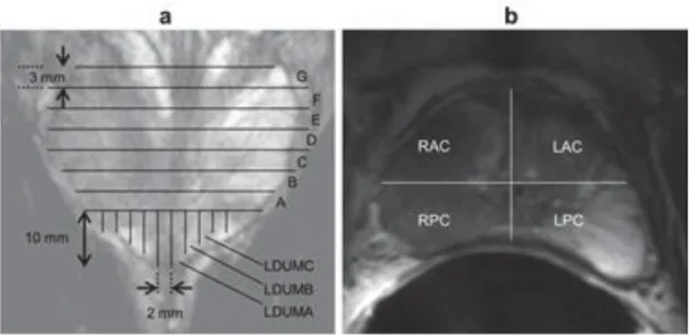
Figure 2.7 Diagrams of pathologic sectioning protocol overlaid on a coronal (a) and axial (b) T2w image. After placing the prostate in the sectioning box, the first cut made is

approximately 0.6 mm from the apex of the gland to create the apical section, with successive axial cuts 3mm apart moving towards the base. The axial cross-sections are

designated by letters “A”, “B”, “C”, etc., depending on the size of the prostate, with “A”

being the most apical slice. Slices are divided into four quarters (b). Each quarter is labeled based on the letter of the slice from which it comes and its position in the slice (e.g. anterior/posterior = A/P and right/left = R/L). After removal from the box, the apical portion is sectioned in 2mm intervals with parallel cuts emanating from the urethra. The

sections near the urethra are labeled “RDUMA” (right distal urethral margin A) and “LDUMA” (left distal urethral margin A). The next two sections from the center are then

labeled “RDUMB” and “LDUMB”, etc. This process continues out to the lateral margins of the apical section. Each slice section is then embedded in a paraffin block and one 4-micrometer H&E-stained slide is prepared from each section and digitized. A pathologist then digitally annotates the prostate capsule (red contour) and cancer regions (brown contour) on each slide.

2.3.2 Digitization

Gross sectioned prostates were subjected to quarter mount histological section (QMHS) pathologic processing. Sections were paraffin embedded, Hematoxylin

(46)

23

and Eosin (H&E) stained, and cut at 4 μm thickness. H&E stained slides were digitized using a whole slide scanner (ScanScope CS, Aperio, Vista, CA).

2.3.3 Annotation

The prostate pseudo-capsule and tumor regions within the digitized sections

were annotated by a board certified pathologist with 15 years’ experience, at 20X magnification (resolution 0.58μm per pixel) using a pen tablet screen (Cintiq

21UX, Wacom, Kazo-shi, Saitama, Japan).

2.3.4 Data Assembly

Digitally annotated QMHS slides were then manually assembled into PWM by aligning the capsule annotations of the quartered pathology sections to form a continuous capsule while minimizing overlap of tissues between the combined sections. Anatomic features in the pathology sections being assembled also aided in aligning the QMHS images (Figure 2.8 a, b).

Figure 2.8 (a) Slides from a complete axial slice are then manually assembled into a PWM by aligning the capsule annotations of the quartered pathology sections to form a continuous capsule while minimizing the overlap of tissues between the combined sections (b).

(47)

24

Chapter 3

LATIS Registration

This chapter is adapted with permission from the following publication: Kalavagunta, C., Zhou, X., Schmechel, S. C. and Metzger, G. J. (2014), Registration of in vivo prostate MRI and pseudo-whole mount histology using

Local Affine Transformations guided by Internal Structures (LATIS). J. Magn.

Reson. Imaging. doi: 10.1002/jmri.24629

This was a collaborative project between Dr Greg Metzger, Dr. Xiangmin Zhou, Dr. Stephen Schmechel and me. My primary role in this project was the development of the Matlab software tools to obtain the necessary inputs for the registration process, perform the registration procedures, visualize the results, validate registration performance and enable the application of all registration results to pathologist annotated cancer regions. Implementation of these procedures and validation was a critical component of the MP-MRI model generation process discussed in Chapter 4.

(48)

25

3.1

Synopsis

A novel registration approach called LATIS (Local Affine Transformation assisted by Internal Structures) for co-registering post prostatectomy pseudo-whole mount (PWM) pathological sections with in vivo MRI (Magnetic Resonance Imaging) images is presented. This study included thirty-five patients with biopsy-proven PCa that were imaged at 3T with an endorectal coil. Excised prostate specimens underwent quarter mount step-section pathologic processing, digitization, annotation and assembly into a PWM. Manually annotated macro-structures on both pathology and MRI were used to assist registration using a relaxed local affine transformation approximation. Registration accuracy was assessed by calculation of the dice similarity coefficient (DSC) between transformed and target capsule masks and least square distance between transformed and target landmark positions. LATIS registration resulted in a DSC value of 0.991±0.004 and registration accuracy of 1.54±0.64 mm based on identified landmarks common to both datasets. Image registration performed without the use of internal structures led to an 87% increase in landmark based registration error. Derived transformation matrices were used to map regions of pathologically defined disease to MRI.LATIS was used to successfully co-register digital pathology with in vivo MRI to facilitate improved correlative studies between pathologically identified features of PCa and MP-MRI.

3.2 Introduction

Multi-parametric maps of anatomic, vascular and metabolic data of the prostate acquired using MP-MRI can yield improved discrimination of the extent and aggressiveness of PCa (66-68). An important step in developing and validating MP-MRI biomarkers to detect the extent and aggressiveness of PCa is the registration of in vivo MR images with histopathological sections obtained from

(49)

26

prostatectomy. This multi-modal registration would enable correlation of MRI with postoperative histopathological determination of extent and tumor grade, and ultimately the molecular assessment of aggressiveness.

There has been much interest in the multi-modal co-registration of prostate MRI with other imaging modalities such as CT for treatment planning (69-72), ultrasound for guiding biopsies (73), and pathology for validation of cancer detection (74). With each combination of source and target data come unique challenges for the registration procedure. In this work, the goal was to register in vivo MRI data obtained with a balloon-type endorectal coil (ERCinMR) with images of pseudo-whole mounts (PWM) constructed from quarter mount histologic sections.

The prostate images from in vivo MRI and pathology possess different amounts of deformation/distortion with respect to each other. For example, after digitally assembling quarter mount histological sections into a PWM, the resulting PWM is different from a true whole mount image in multiple ways, including: (a) the boundary shape of the prostate, (b) the unfilled space or gaps between the quarter mount histological sections, and (c) deformation/distortion of each individual quarter. Additionally, the difference between the ERCinMR and the tissue observed on pathology is a result of multiple factors, including: (a) physical distortion of the prostate due to the presence of the inflated endorectal coil, (b) deformation of the tissue after excision and (c) shrinking of the tissue due to fixation. Without completely characterizing all the intermediate deformations, the registration procedure described in this work focuses on directly registering ERCinMR with PWM images due to the fact that both data sets are readily available, and characterization of the intermediate deformations are not easily obtainable.

LATIS is a technique that uses a relaxed Local Affine Transformation approximation assisted by the identification of large Internal Structures. In LATIS, the prostate capsule and large internal anatomic structures are used as

(50)

27

constraints for registration. This technique does not require the accurate definition of a set of multiple paired landmarks between the source and target data which are difficult to obtain in general and the basis for leading registration methods tackling similar problems. The large structures are, arguably, easier to manually identify on both pathology and MRI and provide a larger continuum of spatial information to guide the registration procedure. In this study, the ability of LATIS to co-register PWM and ERCinMR images is evaluated, and the use of this registration to map regions of pathologically identified cancer onto the in vivo MRI is demonstrated.

3.3 Methods

Data used in this study was obtained from patients with biopsy-proven prostate cancer (35 men, age range 50-73 years, mean age 62 years) after obtaining written signed consent for a study reviewed and approved by the local Institutional Review Board.

3.3.1 In Vivo MR Data

In vivo MR data was obtained from the T2-weighted (T2w) axial MR images. The

axial images were positioned such that the slice plane passed perpendicular to the posterior surface of the prostate (See Chapter 2 Sections 2.2.1 to 2.2.3).

(51)

28

Figure 3.1 A schematic demonstrating the procedure to co-register pathology to T2w

MRI using LATIS. First, the source (a) and target (b) images are segmented, scaled and translated. Second, the prostate capsule and internal structure masks are identified to constrain the pathology transformation. The source and target masks (d and e) are registered and a transformation matrix is obtained. Images (c) and (d) show the transformation flow matrix and applied deformation field respectively. Third, the transformation matrix is applied (red arrow) to the pathology (f) which places it in spatial correspondence to the T2w MRI resulting in (g).Lastly, applying the transformation matrix to each one of the annotated cancer regions (i) places them in the spatial framework of the anatomic T2w images (j).

3.3.2 Pathology Data

Excised prostates were formalin fixed, gross sectioned, paraffin embedded, cut

at 3 μm, H&E stained, digitized, annotated by an experienced pathologist and

(52)

29

based on a special sectioning box (Figure 2.6). Vertical slits in the box, 3 mm apart, allowed the consistent parallel sections to be cut perpendicular to the posterior surface of the prostate with a thickness of 3 mm to match the orientation and thickness of the axial ERCinMR slices. Positioning both the imaging and sectioning planes perpendicular to the posterior surface of the prostate was the method we used to get slices which matched as closely as possible. From the assembled PWM, binary masks of both annotated tumor regions and the prostate capsule were generated (Figure 3.1). For each patient, a single PWM at the center of the index lesion was chosen for registration (Chapter 2 Section 2.3).

3.3.3 Image Registration

In order to register the PWM (source image) to the ERCinMR (target image) (Figure 3.1), a transformation that can map the source image to the target image must be found. Since the source and target image belong to two completely different imaging modalities, a direct mapping relationship between these two images cannot be readily established without additional inputs or modifications. The first step in the process involved manually converting the source and target into tri-intensity grayscale images (Figure 3.1) such that the internal structures had a grayscale value of 128 and the rest of the prostate has a value of 255. This created the potential for developing a direct mapping between the two datasets. To register the two tri-intensity grayscale images, some assumptions are introduced:

1. The 2-dimensional source and target images correspond to the same cross-section of the prostate in terms of the position and the outward normal direction.

(53)

30

2. There exists a path-independent, unique mapping between the source and the target image.

3. The image intensity between the source and target image is conserved.

These three assumptions are reasonable and can be easily satisfied in most cases. The first assumption is met by the standard data collection and sectioning protocols employed in this study. This condition is of the upmost importance because, as the source and target images diverge in terms of their spatial correspondence, there is decreasing benefit to perform the registration since the cancer region annotated in the source image cannot be guaranteed to exist in the target image.

The second assumption establishes that the problem is well-posed. Supposing assumption No.1 holds, there exists a mapping relation between the source and target images as they both represent different realizations of the same cross-section of the prostate. Employing a linear approximation for the mapping will guarantee a unique and path-independent solution. The existence of a solution and its uniqueness establish that the problem is well-posed (75), hence the solution is guaranteed.

The third assumption forms the basis for the image registration procedure. With assumption No. 1, both the source and the target images are referring to the same cross-section of the prostate but differ due to in-plane deformation. After converting the source and target images to the tri-grayscale-images, the intensity conservation principle (76) is readily applicable and a relationship can be established between the source and target images. With this established relationship, the mapping relation between the source and target image can subsequently be derived with the help of assumption No. 2. The derivation is shown in next section. In summary, although three assumptions were introduced, assumption No. 1 is the most fundamental. If assumption No. 1 is achievable,

(54)

31

assumptions No. 2 and 3 are imposed, both of which serve as a foundation for the following registration derivation.

3.3.4 Theory

Let I(x, y, t) be the intensity of an image, which is a function of space and time.

When the source and the target tri-grayscale-images are treated as the images of a deforming prostate at two different time points, time is involved. Therefore, one can assign the source image at t1 and assign the target image at t2.

Following assumption No.1, assumption No. 3 imposes the intensity conservation principle which implies that the total derivative of the intensity is invariant, i.e.

݀ܫሺݔǡ ݕǡ ݐሻ

݀ݐ ൌ ͲǤ

(3.1)

Expanding the left hand side (LHS) of the equation, it becomes ݀ܫሺݔǡ ݕǤ ݐሻ ݀ݐ ൌ ߲ܫሺݔǡ ݕǡ ݐሻ ߲ݔ ݀ݔ ݀ݐ൅ ߲ܫሺݔǡ ݕǡ ݐሻ ߲ݕ ݀ݕ ݀ݐ ൅ ߲ܫሺݔǡ ݕǡ ݐሻ ߲ݐ ൌ ܫ_ǡ௫ݔᇱ_{൅ ܫ} ǡ௬ݕᇱ൅ ܫǡ௧ ൌ ͲǤ (3.2)

According to assumption No. 2, there exists a transformation such that the above equation (3.2) is satisfied. Since this exact transformation is unknown, the assumption of a local affine transformation is made between the source and target image, which is,

൥ݔ෤ݕ෤ ͳ ൩ ൌ ൥ ߠ ߠ ܮ_௫ െ ߠ ߠ ܮ௬ Ͳ Ͳ ͳ ൩ ቈ ݔ ݕ ͳ቉ (3.3)

where ሺݔǡ ݕሻ represents the source image at t1, ሺݔǡ෥ ݕ෤ሻ represents the target image

(55)

32

affine transformation is a proposed approximation, a more relaxed linear approximation can be adopted, namely,

൥ݔ෤ݕ෤ ͳ ൩ ൌ ൥ ܽ_ଵ ܽ_ଶ _ܽ_ଷ ܽ_ସ ܽ_ହ _ܽ_଺ Ͳ Ͳ ͳ ൩ ቈ ݔ ݕ ͳ቉ (3.4)

which relaxes the T constraint between the transformation parameters ሼܽଵǡ ܽଶǡ ܽସǡ ܽହǡ ܽ଺ሽ. This linear approximation satisfies assumption No. 2. With respect to the approximation, there is no qualitative difference between equation (3.3) and equation (3.1) since they are both linear functions but, as shown in a later part of this section, it is desirable to select equation (3.1) over equation (3.3) to reduce the correlation between the transformation parameters resulting in a simpler solution procedure. Substituting equation (3.1) into equation (3.2) leads to the LHS not being equal to zero because equation (3.1) is an approximation and an approximations result in errors. Therefore, locally, we have an error function in terms of ሺݔǡ෥ ݕ෤ሻ whereܫሚ_௫, ܫሚ_௬, and ܫሚ_௧ are functions of ሺݔǡ෥ ݕ෤ሻ, which states that

݁ሺܽଵǡ ܽଶǡ ܽଷǡ ܽସǡ ܽହǡ ܽ଺ሻ ൌ ܫሚ௫ݔ෤ᇱ൅ ܫሚ௬ݕ෤ᇱ൅ ܫሚ௧ (3.5)

Now the objective of the registration process is to find a set of transformation parameters ܽԦ ൌ ሺܽଵǡ ܽଶǡ ܽଷǡ ܽସǡ ܽହǡ ܽ଺ሻ் such that error function e is equal to or is minimal with respect to zero. In order to seek the solution for the transformation parameters, a quadric error functional is constructed as

ȫ ൌͳ

ʹ்݁݁Ǥ

(56)

33

Further taking the variation of the quadratic functional, yields,

ߜȫ ൌ߲ȫ

߲ܽԦߜܽԦ ൅

߲ȫ

߲ܽԦ_௜ߜܽԦ௜൅ ڮ ݄݄݅݃݁ݎ݋ݎ݀݁ݎݐ݁ݎ݉ݏ

(3.7)

Since the transformation parameters are constants, the higher order terms vanish after taking the first variation of the quadratic functional, i.e. ܽԦ௜ ൌ Ͳ, for all

i > 1. And according to the Ekeland’s variational principle (77), there exist a solution for ܽԦ such that ߜȫ ൌ Ͳ which corresponding to the minimization of the error function e. Since ߜܽԦ is arbitrary and is not always equal to zero, the only possibility to yield ߜȫ ൌ Ͳ is that the following equation is always satisfied,

ͲሬԦ ൌ ߲ȫ ߲ܽԦ ൌ ்߲݁ ߲ܽԦ ݁ ൌ ܿԦሺܿԦ்ܽԦ െ ݂ሻሺܿԦ்ܽԦ െ ݂ሻ (3.8) Where ܿԦ் _{ൌ ൫ݔ෤ܫሚ} ௫ݕ෤ܫሚ௫ܫሚ௫ݔ෤ܫሚ௬ݕ෤ܫሚ௬ܫሚ௬൯ (3.9) ݂ ൌ ݔ෤ܫሚ௫൅ ݕ෤ܫሚ௬൅ ܫሚ௧ (3.10)

Therefore, the transformation parameters can be solved from the following equation

ܿԦܿԦ்_{ܽԦ ൌ ܿԦ݂ǡ} _(3.11)

where the resulting transformation parameters are the optimal solution satisfying equation (3.2) and subsequently, provides the transformation satisfying equation (3.1).

(57)

34

A pixel by pixel solution of the transformation parameters is computationally expensive and may be ill-posed in the sense of Hadamard(75). For reducing the computational cost, the tran