Detecting potholes with monocular computer vision: A Performance evaluation of techniques

(1)

computer vision: A performance

evaluation of techniques

By

Sonja Nienaber

Thesis presented in partial fulfilment of the requirements for the degree Master

of Science in Engineering at the University of Stellenbosch

Supervisor: Dr. MJ Booysen

Department of Electrical & Electronic Engineering, Stellenbosch University Co-supervisor: Dr. RS Kroon

Computer Science Division, Stellenbosch University

(2)

ii

DECLARATION

By submitting this thesis electronically, I declare that the entirety of the work contained therein is my own, original work, that I am the sole author thereof (save to the extent explicitly otherwise stated), that reproduction and publication thereof by Stellenbosch University will not infringe any third party rights and that I have not previously in its entirety or in part submitted it for obtaining any qualification.

Date: . . . March 2016. . .

(3)

iii

ABSTRACT

Potholes in road surfaces create problems for motorists and driverless vehicles. This is because the damage to the vehicle that can be caused by hitting a pothole with a vehicle can be costly and even dangerous. Previous works of other authors with respect to pothole detection did not investigate the limitations of the detection capabilities of their works such as the distance at which the potholes could be detected and often used footage where the camera was directly facing the road, thereby only having a viewing range of roughly 2-4 m.

In order to complete this project, it was necessary to obtain suitable footage of potholes. The method for collecting the pothole footage can be seen as novel. The method included attaching a GoPro camera inside of a vehicle windscreen and photographing the road as the vehicle was driven around. This footage is, therefore, akin to a driver’s viewpoint of the road. This viewpoint is advantageous as it ensures that the maximum amount of the road can be photographed by the camera. By mounting the camera in this manner, it could potentially be possible to detect potholes before the vehicle reaches them as opposed to other works done where the camera was mounted to the rear of the vehicle. In the instance of a driverless vehicle, this would allow the vehicle to avoid hitting the pothole and would prevent damage to the vehicle.

Due to the difficulty of detecting potholes, the footage was split into two different datasets namely, a simple scenario and a complex scenario. The simple scenario considered footage where the road lighting conditions were always open and clear. In this scenario, the road was extracted and only the extracted region was used in pothole detection algorithms. The complex scenario considered footage where the road lighting conditions were either open or contained mixed lighting conditions. Therefore, in this scenario, the input images were cropped to the suspected road region within the image. This region is rectangular and contains additional information along the sides of the image such as foliage etc.

Image processing algorithms, as well as machine learning algorithms were deployed in this thesis to investigate the feasibility of pothole detection. The machine learning algorithms used, consisted of an LBP (Local Binary Pattern) cascade classifier and an SVM (Support Vector Machine) with HOG (Histogram of Oriented Gradients) features.

The pothole locations were also analysed in terms of the relative distance that a pothole occurred from the camera. This process is known as depth estimation in monocular images, and

(4)

iv

this work allowed for determining the ranges at which pothole detection was more successful than others. The discrepancy in the results at the different depth ranges might indicate that different algorithms and classifiers need to be implemented for different ranges to increase the performance of the pothole detector.

The final results of this project indicate that under certain conditions, it is possible to detect potholes with modest results.

(5)

v

UITTREKSEL

Slaggate in die pad skep probleme vir motoriste en bestuurderlose voertuie. Dit is omdat die skade wat veroorsaak kan word aan die voertuig deur 'n slaggat te slaan duur en selfs gevaarlik kan wees. Vorige werke van ander skrywers met betrekking tot slaggat opsporing, het nie die beperkinge van die opsporing vermoëns van hul werke ondersoek nie soos byvoorbeeld, die afstand wat die slaggate kon opgespoor word en dikwels was beeldmateriaal gebruik waar die kamera direk na die pad kyk en sodoende net besigtiging van ongeveer 2-4 m het.

Ten einde hierdie projek te voltooi, was dit nodig om geskikte beeldmateriaal van slaggate te bekom. Die metode vir die insameling van die slaggat beeldmateriaal kan gesien word as nuut. Die metode behels die hegting van 'n GoPro kamera aan die binnekant van 'n voertuig voorruit en om dan die pad fotografeer soos wat die voertuig bestuur word. Hierdie materiaal is dus soortgelyk aan die oogpunt van 'n bestuurder. Hierdie metode is voordelig aangesien dit verseker dat die maksimum area van die pad gefotografeer kan word deur die kamera. Deur die kamera te monteer op hierdie wyse, kan dit potensieel moontlik wees om slaggate op te spoor voordat die voertuig hulle bereik, in teenstelling met ander werke gedoen waar die kamera aan die agterkant van die voertuig gemonteer was. In die geval van 'n bestuurderlose voertuig, sou dit die voertuig in staat stel om slaggate te vermy en gevolglik skade aan die voertuig te voorkom.

As gevolg van die probleme van die opsporing van slaggate, was die beeldmateriaal verdeel in twee verskillende datastelle naamlik 'n eenvoudige geval en 'n komplekse geval. Die eenvoudige geval oorweeg beeldmateriaal waar die pad altyd oop en duidelik was. In hierdie geval, is die pad onttrek en slegs die onttrekde streek is gebruik om slaggate in op te spoor. Die komplekse geval oorweeg beeldmateriaal waar die pad omstandighede of oop of gemengde lig omstandighede gehad het. Daarom, in hierdie geval, was die beelde geknip om die vermeende pad streek binne die beeld uit te haal. Hierdie streek is reghoekig en bevat aanvullende inligting langs die kante van die beeld soos blare en bome.

Beeldverwerking algoritmes, asook masjien leer algoritmes is ontplooi in hierdie verhandeling om die haalbaarheid van slaggat opsporing te ondersoek. Die masjien leer algoritmes wat hier bruik word, bestaan uit 'n LBP (Local Binary Pattern) kaskade klassifiseerder en 'n SVM (Support Vector Machine) met HOG (Histogram of Oriented Gradients) kenmerke.

Die slaggate is ook ontleed in terme van die relatiewe afstand wat 'n slaggat plaasgevind vanaf die kamera. Hierdie proses staan bekend as diepte skatting in monokulêre beelde. Hierdie werk het dit moontlik gemaak om te bepaal hoe suksesvol die slaggat opsporing was met

(6)

vi

betrekking tot die afstand waar die slaggat voorkom per klassifiseerder. Die verskil in die resultate van die verskillende diepte reekse kan dui dat verskillende algoritmes en klassifiseerders nodig is vir verskillende reekse om die prestasie van slaggat opspoorders te verbeter.

Die finale uitslae van hierdie projek dui aan dat onder sekere omstandighede, is dit moontlik om slaggate op te spoor met 'n beskeie resultate.

(7)

vii

PUBLICATIONS

The following publications were made from the work presented in this thesis:

 S.Nienaber, M.J. Booysen, R.S. Kroon. “Detecting potholes using simple image processing techniques and real-world footage”, 2015 South African Transport Conference (SATC), July 2015, Pretoria, South Africa.

 S. Nienaber, R.S. Kroon, M.J. Booysen, “A Comparison of Low-Cost Monocular Vision Techniques for Pothole Distance Estimation”, IEEE Symposium on Computational Intelligence in Vehicles and Transportation Systems (CIVTS), December 2015, Cape Town, South Africa.

Two annotated pothole datasets were created for this project and is freely available online at: http://goog.gl/Uj38Sf.

(8)

viii

ACKNOWLEDGEMENTS

I would like to thank the following people and entities for their assistance:

 My mother for her emotional support and encouragement during the entire duration of the degree.

 Jenna for late night phone calls of encouragement during the all-nighters.

 Dr. MJ Booysen. I would like to thank him for taking me as one of his students and giving me the opportunity to go overseas for an internship.

 Dr. RS Kroon, for his assistance throughout the year and especially the corrections to the thesis document.

 Dr. W Brink for his assistance with the depth estimation work.

 Prof. BM Herbst for his general advice with respect to machine learning as applied to computer vision.

 Prof. TR Niesler for letting me borrow one of his DSP lab computers for the duration of the project.

 Prof. K Jenkins for his insight into the physical aspects of the formation of potholes.  MTN for providing me with financial support for the project.

(9)

LIST OF FIGURES

Figure 1.1.1 Example typical pothole photos. ... 4

Figure 2.2.1 HSV colour space illustration ... 11

Figure 2.2.2 Light intensity change for various colour schemes ... 11

Figure 2.2.3 Example normalised Gaussian kernel ... 13

Figure 2.2.4 Visual illustration of a Gaussian kernel... 13

Figure 2.2.5 Sobel operator in mask form ... 16

Figure 2.2.6 Example convex hull algorithm ... 17

Figure 2.3.1 LBP Feature illustration ... 19

Figure 2.3.2 LBP lighting variations example ... 20

Figure 2.3.3 HOG feature descriptor extraction ... 21

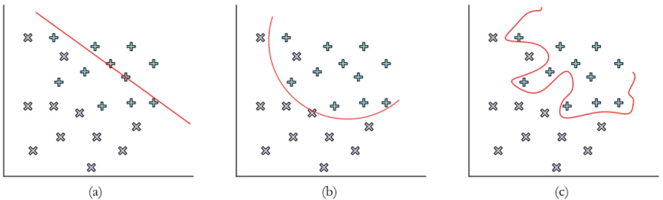
Figure 2.4.1 Graphs to show underfitting (a), good fit (b) and overfitting (c) ... 23

Figure 2.4.2 Cascade classifier working ... 24

Figure 2.4.3 SVM hyperplane illustration ... 26

Figure 2.4.4 Sliding window functioning ... 30

Figure 2.4.5 Image pyramid example with scale set to 50% ... 31

Figure 3.4.1 Input data pre-processing ... 42

Figure 3.7.1 Illustration of (a) the pinhole camera model and (b) the corresponding camera plane and image co-ordinate systems ... 50

Figure 3.7.2 Camera calibration ... 52

Figure 3.7.3 Fisheye distortion illustration ... 52

Figure 3.7.4 Fisheye correction measurements... 53

Figure 3.7.5 Similar triangles illustration ... 55

Figure 3.7.6 Cross ratio point mapping ... 56

Figure 3.7.7 Results of the various approaches ... 60

Figure 3.7.8 Results of the various approaches at 4.93 m to the left of the camera ... 61

Figure 3.7.9 Cross ratio comparisons ... 62

Figure 4.2.1 Road extraction algorithm example... 67

Figure 4.3.1 Pothole detection algorithm ... 69

Figure 4.4.1 Simple scenario dataset pothole content breakdown. ... 71

(14)

v

Figure 4.4.3 HOG features visualisation ... 73

Figure 5.3.1 Example of the effect of grouping detections ... 83

Figure 5.4.1 Image processing simple scenario precision/recall curves ... 84

Figure 5.4.2 Image processing complex scenario precision/recall curves ... 85

Figure 5.5.1 LBP simple scenario classifier precision/recall curves ... 86

Figure 5.5.2 LBP complex scenario classifier precision/recall curves ... 87

Figure 5.6.1 SVM+HOG simple scenario classifier precision/recall curves ... 88

Figure 5.6.2 SVM+HOG complex scenario classifier precision/recall curves ... 89

Figure 5.7.1 Maximum F1-score classifiers for the simple scenario ... 90

Figure 5.7.2 Maximum F1-score classifiers for the complex scenario ... 90

Figure 5.7.3 Example output of machine learning classifier in simple scenario. ... 92

Figure 5.7.4 Example output of machine learning classifier in complex scenario. ... 92

Figure 5.8.1 Simple depth estimation results ... 94

(15)

LIST OF TABLES

Table 2.5.1 CDDMC algorithm results. ... 35

Table 2.5.2 Experimental Setup Done by Koch and Brilakis ... 36

Table 2.5.3 Kinect Sensory Key Properties. ... 38

Table 3.6.1 Sample summary ... 46

Table 4.4.1 HOG descriptor parameter values ... 74

Table 5.7.1 Optimal classifier settings and performance based on F1-score ... 91

Table 5.8.1 Detected potholes expressed as a percentage as a function of depth... 96

(16)

ABBREVIATIONS AND ACRONYMS

ANN – Artificial Neural Network

CDDMC – Critical Distress Detection, Measurement and Classification DFS – Distress Frame Segmentation

fps - Frames Per Second

GPR - Ground Penetrating Radar GPRS – General Packet Radio Service GPS - Global Positioning System

HOG – Histogram of Oriented Gradients HSV – Hue, Saturation, Value

IR – InfraRed

LASER - Light Amplification by the Stimulated Emission of Radiation LBP – Local Binary Pattern

LCD – Liquid Crystal Display LOO – Leave-one-out

LRF – Laser Range Finder LUT – Look Up Table

MLP – Multi-Layer Perceptron RBF – Radial Basis Function RGB – Red, Green, Blue

ROC – Receiver Operating Characteristic

SANRAL - South African National Roads Agency Limited SIFT – Scale-Invariant Feature Transform

SURF – Speeded-Up Robust Features SVM – Support Vector Machine

(17)

4

CHAPTER 1 INTRODUCTION

1.1 BACKGROUND

In modern day society, tarred roads have become critical for services and goods to be available to citizens as well as to cater to their transportation needs. The cost of building a tar road is estimated to be up to R 25 million per kilometre [1] and is an expensive necessity. As the demand for food and products to be available across a country increases, the logistical challenges of transporting these items increases, leading to more heavy motor vehicles using the roads. Heavy motor vehicles such as trucks used by freight operators are the biggest culprits in damaging the road surface due to their heavy weight and high axle load. The term axle load is used to describe the force that is exerted on the pavement by a vehicle and is one of the most important considerations when designing a road. A 22 m long heavy motor vehicle can have a load of up to 35 tons [1], which has a larger axle load than a light motor vehicle. One type of damage that is created over a period of time is known as potholes. Two different examples of potholes found in suburban areas are given in Figure 1.1.1.

Figure 1.1.1 Example typical pothole photos. In these photos, several different types of potholes can be seen and in a variety of lighting conditions.

The manner in which a pothole forms is dependent on the type of bituminous pavement surfacing. The volume of traffic and the axle load experienced by the road are example factors that lead to fatiguing of the road surface, resulting in the formation of cracks. These cracks allow

(18)

5

water to seep through and mix with the asphalt. When a vehicle drives over this area, this water is expelled through the crack with some of the asphalt, and this will slowly create a cavity underneath the crack. Eventually the road surface will collapse into the cavity, resulting in a visible pothole. If regular road maintenance is neglected, the aforementioned cracks are not repaired before they cause substantial damage to the road. Therefore, potholes usually increase in number during and after heavy rainfall seasons [2].

There are sophisticated commercial products available on the market that will scan the road for all types of distress and log the findings for maintenance purposes, such as Roadscanners [3]. These types of vehicles are fitted with a 3D accelerometer, 2D laser scanner, video camera, thermal camera and 3D Ground Penetrating Radar (GPR). All of this adds up financially to a substantial amount and it is therefore normally only large agencies like the South African National Roads Agency Limited (SANRAL) that can afford to purchase these types of vehicles. SANRAL is responsible for the maintenance and planning of the highways in South Africa; therefore, highways tend to be in better condition than municipal roads. Equipment such as a Roadscanner vehicle remains out of reach for municipalities with smaller budgets. This leaves manual pothole detection in towns as the only viable option at this point in time, thereby establishing a need for an inexpensive and accurate pothole detection method that can assist in automating the process.

1.2 PURPOSE OF THE PROJECT

The purpose of this project is to investigate the feasibility of automatically detecting potholes with a digital camera. Therefore, a visual approach is required and the images are processed off-line with several different algorithms. The algorithms that are investigated are image processing algorithms, as well as machine learning algorithms. If potholes can be detected, more expansive applications could use this information and incorporate the pothole detection system with other types of technology such as GPRS (General Packet Radio Services) and GPS (Global Positioning System) to log these potholes for maintenance purposes. If the pothole algorithms are found to perform fast enough, it would then also be possible to add a pothole detection feature to driverless vehicles [4, 5].

(19)

6

1.3 RESEARCH OBJECTIVES

The research objectives of this investigation are rooted in the assumption that pothole regions can be distinguished from non-pothole regions in an image. The degree to which this statement is true, will be determined. The investigation will be conducted on a simple scenario and a complex scenario. The simple scenario can be considered to be the ideal case where only open and clear road images are used and therefore the road can be extracted. In the complex scenario, the real-world conditions which include mixed lighting conditions prevented the road from being extracted. Therefore, these images contained foliage and other objects. Three different approaches will be evaluated to analyse the different scenarios, namely an algorithmic image processing approach, and two machine learning approaches.

Research objective 1:

To investigate the feasibility of detecting potholes in images. Two types of images will be evaluated: a simple scenario and a complex scenario.

To compare the results between an approach using classical image processing algorithms and two suitable machine learning algorithms.

To quantify the effect that potholes have at different distances from the camera on the performance of each of the classifiers.

(20)

7

1.4 SCOPE OF WORK

This study investigates how effectively potholes can be detected by using a visual approach i.e. a camera. This approach required that the camera be mounted to the inside of the windscreen, facing the road. The windscreen of the vehicle was cleaned regularly and therefore the assumption is made that there are no dirty spots on the windscreen, and subsequently, in the images. Due to the physical and visual nature of the problem, only pothole footage during either sunny or cloudy conditions are considered, but not during rainy conditions.

Machine learning algorithms, especially when applied to high-resolution images, can be a very time-consuming task and therefore it was decided to only investigate the LBP (Local Binary Patterns) cascade classifier and the SVM (Support Vector Machine) with HOG (Histogram of Oriented Gradients) classifier. These classifiers are known to have a much shorter training time than that of, for example, a Haar cascade classifier, which is more suited to the time period of the project. Preliminary work where a Haar cascade classifier was trained required seven weeks to complete.

1.5 THESIS STRUCTURE

The structure of the rest of this thesis is as follows:

 Chapter 2: Literature review. Sections 2.2 – 2.4 of this chapter focusses on explaining the technical detail of the various methods and algorithms used to detect potholes in this thesis. Section 2.5 discusses the various existing works available in the academic community with regards to pothole detection.

 Chapter 3: Data set collection and preparation. Sections 3.2 explains how the data was obtained for this project. In Section 3.3, it is discussed that two individual investigations take place in this study namely, a simple scenario and a complex scenario. In the simple scenario, clear open roads are used and the road region within the image is extracted by using the colour of the road before the potholes are detected. In the complex scenario, however, the conditions were varied to include open and mixed lighting conditions. Therefore, the road could not be

(21)

8

extracted by its colour and the images were cropped to the region in the image where the road is expected to be. This scenario best represents the expected real-world pothole detection problem. The necessary steps to pre-process the data before training/testing could be done is discussed in Section 3.4. Section 3.5 discusses the manner in which the data is annotated, especially for training purposes. The actual number of positive and negatives samples use in the investigation is tabulated in Section 3.6. As it was decided that the specific range in which the pothole detection solution can detect potholes needed to be evaluated, it was necessary to compare different depth estimation techniques in monocular images. This work is presented in Section 3.7.

 Chapter 4: Development and methodology. The method for extracting the road surface based on its colour is discussed in Section 4.2. The development of the image processing pothole detection algorithm is discussed in Section 4.3. The methodology that was followed to determine the finer details necessary in the design of the machine learning is discussed in Section 4.4 and 4.5. The machine learning classifiers that are used in this investigation are LBP cascade classifiers and SVM with HOG features classifiers.

 Chapter 5: Results. Section 5.2 discusses the performance metric used to compare the various classifiers’ performance was selected as precision/recall curves. In Section 5.3 the specific setup used in OpenCV to utilize the machine learning functions is discussed. The remaining sections of Chapter 5 presents the performance results of the classifiers and compares them to one another per scenario being investigated. The classifiers are also evaluated based on the relative distances at which the classifiers could detect potholes (Section 5.8). Lastly, the performance of the classifiers was timed and analysed in Section 5.9.

 Chapter 6: Conclusion and recommendations. In the last chapter, the final conclusions that were found during the course of the project based on the results presented in Chapter 5 is given. Lastly, recommendations for improvement and future work are also given and explained.

(22)

9

CHAPTER 2 LITERATURE REVIEW

2.1 INTRODUCTION

This chapter reviews the relevant literature with respect to the image processing algorithms and machine learning algorithms applied in this thesis. The image processing algorithms/techniques discussed are usually only applicable to single channel (for example, the red colour matrix in an RGB image). If it is necessary to apply these algorithms to a full RGB image, the image must first be split into its three respective channels, the algorithm applied to each channel respectively, and the results are merged together to create the new RGB image.

The algorithms and techniques are divided and discussed in different sections. Section 2.2 contains the necessary theory to understand the image processing methodology used in Chapter 4. This includes information regarding the colour space, edge detection and noise removal techniques used. The operation of the contour detection and convex hull algorithm is also discussed in Section 2.2. In Section 2.3, the various types of features used are explained. After Section 2.3, the specific machine learning algorithms are explained in Section 2.4. The two different types of machine learning algorithms that will be used in this project is a cascade classifier and an SVM (Support Vector Machine). The theory with respect to the application of the machine learning algorithms such as the sliding window and image pyramid techniques, is also discussed. Due to the fact that features can also be used in the absence of machine learning to detect objects, these sections are separated. In Section 2.5, the papers that are directly involved with pothole detection are discussed. From the papers it was found that various technologies can be applied to pothole detection such as accelerometers to measure the vibrations of the vehicle and infra-red cameras that obtain depth maps of an area. Lastly, a conclusion regarding all of the theory is presented in Section 2.6.

Note that all of the algorithms were implemented by using OpenCV 2.4.8 [6] which is an open-source computer vision library. For practical purposes, it is also important to note that in OpenCV, the top left pixel is the reference point and is therefore (x,y) = (0,0). If a pixel’s colour

(23)

10

is black, the value in OpenCV is 0 and if a pixel is white, its value is 255. Where applicable in this chapter, as well as the rest of the thesis, this information should be kept in mind.

2.2 IMAGE PROCESSING

This section contains the relevant image processing theory necessary for the comprehension of the image processing algorithm developed in Chapter 4.

2.2.1 COLOUR SPACES

The term colour space refers to the collective term to describe the particular mathematical representation of the different colours as well as their saturation and contrast [7]. The RGB (Red, Green, Blue) colour space consists of a red, green and blue channel and is very commonly used to represent images in a variety in applications, such as LCD (Liquid Crystal Display) screens [8]. A colour channel can be thought of as a matrix containing the exact pixel values for each of the primary components of the chosen colour model [9]. In general, a colour space consists of three different channels. The RGB colour space is not appropriate when processing images, because it is difficult to discriminate between the different colours [10]. A much more suitable colour space is the HSV (Hue, Saturation, Value) colour space as it separates the chroma (colour information) from the luma (intensity information) in the channels which in turn can simplify the task of detecting objects within an image [11]. An example illustration of this colour space is shown in Figure 2.2.1. From the figure, it is clear that the colour space uses a conical shape to represent the various colours. The hue is expressed on a circular scale and is therefore either represented in degrees or radians. The saturation is expressed as the radius of the cone at a particular height from the vertex of the cone, while the value channel is expressed in terms of the height of the cone. HSV performs well in conditions where there is a high variety in light intensity and can be observed in Figure 2.2.2 [12]. In the figure, the light intensity was varied and is was found that by using the HSV colour space the colours of the image could be more accurately extracted than in the RGB colour space.

(24)

11

Figure 2.2.1 HSV colour space illustration [13]. The colour space has a conical shape which separates the colours more evenly than the RGB colour space. Hue is measured on a circular scale and is indicated in either radians or degrees. The saturation value is measured with respect to the centre of the cone and is akin to its radius at a particular height from the vertex of the cone. The light intensity is represented by the value and is measured from the tip of the cone to the particular colour.

The HSV colour space does, however, not perform well if the colour of the object that needs to be detected varies over a wide range. For example, HSV is not the best suited colour space to detect objects that are orange and have a wide range of saturation for the object.

Figure 2.2.2 Light intensity change for various colour schemes [12]. A variety of colour spaces are weighed against each other over change in intensity. The only colour spaces implemented in OpenCV are the RGB and hue colour spaces. From the figure, the hue channel remains much more correct for a wider range than for the RGB colour space.

(25)

12

However, in this project, the colour information of the pothole is not used to detect the pothole, therefore, the HSV spectrum is a suitable choice.

2.2.2 NOISE REMOVAL TECHNIQUES IN IMAGES

This section discusses the different noise removal techniques used in this thesis namely: Gaussian blur and morphological operations such as erosion and dilation.

2.2.2.1 GAUSSIAN BLUR

Blurring is a method for smoothing images to remove noise [14]. There are many different types of kernels that can be used to smooth an image such as average (also referred to as a box filter), median and Gaussian. Each type of blurring function uses a kernel to scan the image and by performing kernel-specific calculations, a smoothed output image is produced. These kernels are usually of the form A x A pixels where A is an odd integer number of pixels. The average kernel calculates the average value of the pixels in the kernel window, normalises the average value and outputs this value to the x- and y-coordinate of the centre pixel of the kernel at the output image. The kernels are normalised to ensure that the output image does not increase in brightness and keeps the colour information accurate [15]. Similarly, the median kernel will use the median value of the kernel to determine the output. A Gaussian kernel uses the Gaussian bell curve to perform its calculations. The Gaussian operator was used in this project as it is required by the Canny edge detector (discussed in the next section).

The Gaussian operator given a two-dimensional space (such as the x- and y-coordinates of a Cartesian plane) is given in equation (2.2-1). The standard Gaussian operator includes a µ, and refers to the position of the centre of the peak, however, in image processing, this parameter does not feature in this equation as the Gaussian bell curve is centred about the origin and is therefore zero [16].

g(x,y) = ce−

(x2+y2)

(26)

13

An example of a normalised 3 x 3 Gaussian kernel is shown in Figure 2.2.3 [16].

Figure 2.2.3 Example normalised Gaussian kernel. The kernel has a size of 3 x 3 pixels and is an example approximation of the Gaussian kernel. Note that to normalise the output of the kernel, the kernel is divided by the sum of the internal components which is 16 for this particular kernel.

The visual representation of a large Gaussian kernel is given in Figure 2.2.4. The smaller picture in the bottom right corner illustrates what the Gaussian kernel intensity values are that will be applied to the pixel regions included in the kernel. The higher the value of the intensity, the lighter the pixel becomes and if the value is smaller, the pixel value becomes darker.

Figure 2.2.4 Visual illustration of a Gaussian kernel [17]. The centre figure illustrates the bell curve that is characteristic of the Gaussian kernel. As the pixel values within an image is discrete, the curve is also discrete. In the bottom right corner, an example of the kernel as it is applied to an image is illustrated.

2.2.2.2 EROSION AND DILATION

There are a variety of morphological operations such as erosion and dilation [18]. The erosion and dilation operations can be used in to remove residual noise from an image that is typically created when edge detection has been implemented [19]. In this project, both erosion and

1 2 1 2 4 2 1 2 1 1

(27)

14

dilation are only applied to binary (black-and-white) images and are therefore discussed in terms of how these two operations function on binary images.

Practically, the erosion binary operation increases the number of black pixels in a binary image while the dilation binary operation increases the number of white pixels. In both operations, there is a kernel that is convoluted with the input image to produce an output [14]. In OpenCV, this kernel has a square shape of size A x A where A is any odd integer above 1.

In the case of the dilation kernel, it effectively scans the pixels of an input image and if there are any white pixels (maximum pixel value) present in the “window” of the kernel, it sets the output pixel at the coordinates of the centre pixel of the kernel, to the maximum pixel value. Similarly, the erosion kernel determines the minimum pixel value. This is illustrated by equation (2.2-2) [14]. In the equation src refers to the input source pixels.

erode(x,y) = min (xk_,yk₎_∈_kernelsrc(x+ x k_{, y+ y}k₎ dilate(x,y) = max (xk_,yk₎_∈_kernelsrc(x+ x k_{, y+ y}k₎ (2.2-2)

2.2.3 CANNY EDGE DETECTION

An edge represents a sharp gradient change between neighbouring pixels. Accurate edge detection in images are important for object detection because if the edges of the objects within an image can be extracted; the shape, area and perimeter of an object can be determined which would aid in the successful detection of a particular object [20]. Once the edges have been detected, it is possible to, for example, detect the contours in an image. This process is referred to as edge tracing and it follows either a clockwise or anti-clockwise approach. By picking a particular edge pixel and determining its next clockwise neighbour, a linked list of the data can be created which will describe a continuous contour. Edge detection is also seen as a form of image segmentation as it can be used to segment the image into different regions [19, 20].

A variety of edge detection algorithms are available such as the Prewitt [21], Roberts cross detector [22], Sobel edge detector [23], Scharr [24] and Canny [25].

(28)

15

1. Detection: The edge detector must not be sensitive to noise and must detect the maximum amount of edges in an image that is possible.

2. Localization: The maximum point of the edge calculation should indicate where the true edge location is.

3. Minimal response: There must be no more than one detected edge per edge present in the image.

Due to the above mentioned criteria, the Canny edge detector was selected for use in this thesis.

There are five steps in the Canny edge detector algorithm namely: smoothing, finding gradients, non-maximum suppression, double thresholding and edge tracking by hysteresis [26].

As was mentioned in the previous section, the standard smoothing method used in conjunction with the Canny edge detector is a Gaussian blur/filter [26, 27].

Then, the edges within images can be determined by determining the rate of change of the gradient with respect to the intensities in an image. A method for calculating the gradient of a function f(x,y) is to determine its derivative which leads to:

∇f(x,y) = (𝜕f 𝜕x,

𝜕f

𝜕y) =(gx, gy) (2.2-3) where the partial derivative of the x- and y-axis pixels are denoted by g_x and g_y. A larger derivative would indicate a sharper edge while a smaller derivative indicates a less sharp edge. A derivative equal to zero indicates no gradient change and therefore no edge is present. The partial derivatives g_x and g_y are vectors and the magnitude and direction of the gradient can be determined simply by ‖∇f(x,y)‖ = √g_x2₊_g y 2 (2.2-4) and Direction = arctan(gy g_x) (2.2-5)

(29)

16

Each of the gradients are calculated by using the Sobel-operator [23] which is given in mask form in Figure 2.2.5. The horizontal gradient operator on the left hand side of the image, detects horizontal edges from left to right while the vertical gradient operator on the right hand side of the image detects vertical edges from the bottom to the top.

-1 0 1 -2 0 2 -1 0 1 1 2 1 0 0 0 -1 -2 -1 Vertical gradient operator Horizontal gradient operator

Figure 2.2.5 Sobel operator in mask form. The gradient is determined separately in the x- and y-direction by using two different operators. The horizontal gradient operator is found on the left hand side and the vertical gradient operator is on the right hand side.

Due to the previously mentioned step, the output of the Canny edge detector can be interpreted as a gradient image. In the gradient image, pixels that are black are pixels that have a low gradient while the white pixels represent pixels with a higher gradient. In this manner, the edges are represented by gradients. The next steps simply add additional robustness to the algorithm according to the previously stated criteria.

The next step in the Canny edge detector, is non-maximum suppression which effectively narrows the detected edges. For each detected edge pixel from the previous steps, the maximum gradient magnitude is determined by evaluating its direct neighbours along the direction of the gradient at that edge pixel and only the pixel with the maximum gradient magnitude is selected. This also sharpens the detected edges output image.

A thresholding algorithm which has two thresholds, one low and one high, is applied. If a pixel gradient is below the lowest threshold, it is discarded and a pixel above the highest threshold is deemed a strong edge. Pixel gradients that fall in between the high and low threshold are deemed weak edges.

The last step performs a hysteresis operation. A hysteresis operation has two threshold values and if an edge value is below the lower threshold, it will reject the edge. Similarly, if an edge value is above the upper threshold, it will accept the edge. In this manner, the hysteresis function

(30)

17

traces out the contour of the edge in such a manner that it fits the edges to a connected pixel line and prevents disconnected lines on a single contour.

2.2.4 CONTOUR DETECTION

A contour in an image is the outline/boundary of an object in the image [14] and as stated in Section 2.1, contours in image processing comprise linked lists of neighbouring pixels. By using, for example, an edge detection technique, the output binary image can be fed to a contour detection algorithm. The algorithm will create closed loop contours as contour objects in the software which will then automatically determine the exact location, length and area of the contour. Naturally, it is possible to have multiple contours in an image. For these cases, OpenCV builds hierarchical structures where each element in the structure refers to a contour. Dependant on the type of structure that the user specifies, it is possible to extract only the smaller contours that are found within a larger contour.

2.2.5 CONVEX HULL ALGORITHM

A convex hull algorithm in image processing constructs a convex polygon by using all of the furthest pixel points of a particular contour. An example application that demonstrates this algorithm is shown in Figure 2.2.6.

Figure 2.2.6 Example convex hull algorithm [14]. A convex polygon is fit to the hand in the figure. Points A-H indicate the valleys that are included in the convex polygon that would not be included in a standard contour detection algorithm.

(31)

18

Each of the indentations of the hand are marked (A-H) and indicate the gaps in the figure with respect to the outlying points. These gaps are included in the convex hull because the convex hull algorithm will connect each of the furthest points together with straight lines and would encompass the entire hand.

2.3 FEATURE TYPES

Features, in terms of images, are seen as points of interest and for a particular set of features to be useful in object detection, it is necessary that the object features need to be consistent across all of the instances of the object in all of the images [28].

Careful consideration must be given when choosing a particular feature type as to whether it is applicable to the object that is desired to be detected. In the case of pothole detection, the pothole itself is usually firstly characterized by a dark/black region (sources) and surrounded by lighter regions. Therefore, features that specialize in gradient changes a.k.a. edge detection are a good option for this particular object.

There are many different types of features that can be investigated. Some, such as SIFT (Scale-Invariant Feature Transform) [29] and SURF (Speeded-Up Robust Features) [30], are bounded by a patent and therefore need to be paid for especially if a commercial product is desired [31]. Therefore, this thesis is limited to features that are free and available within OpenCV.

In OpenCV, there are Haar [32], LBP (Linear Binary Pattern) [33] and HOG (Histogram of Oriented Gradients) features [34, 35]. Both the Haar features and the LBP features are known to not be rotation invariant [36, 37]. Therefore, these features are not designed for objects that have a high variety in their rotation in the image. HOG features were specifically developed to detect humans in images, with the emphasis on being able to detect humans in a variety of different poses and in different situations/backgrounds. HOG features, therefore, specialise in detecting objects with a high variety in shape which implies that these features could be a good set of features to consider when detecting potholes as potholes vary greatly in shape.

Initial tests done in this works indicated that the process of training a cascade classifier using Haar features on high-resolution images required upwards of six weeks. Therefore, due to time constraints, these features were excluded from the investigation.

(32)

19

2.3.1 LOCAL BINARY PATTERNS

In [33], LBP (Local Binary Patterns) features were first presented. LBP features are texture operators functioning in a two-dimensional space and can therefore be used to extract texture features in images. The textures in an image can be described as particular patterns present in an image such as a checkerboard pattern or the ridges found in fingerprints. LBP features are determined by thresholding the 8 nearest neighbours around a pixel by the centre pixel’s value. Any value equal to or below the centre pixel is deemed a zero and if the value is higher than the value of the centre pixel, the new value becomes 1. An example of this thresholding transformation of pixels is demonstrated in Figure 2.3.1 by using a 3 x 3 window.

2 4 2 1 3 9 1 7 6 0 1 0 0 1 0 1 1 Transform

Figure 2.3.1 LBP Feature illustration. On the left hand side, there is a sample of 3 x 3 pixels in a window. By using the centre pixel as the threshold, the transformed output window on the right hand side is generated.

The binary interpretation of the output (starting in a clockwise motion from the top left pixel) yields an 8-bit code of 01011100. The 8-bit code is then used and the number of transitions from zero to one is counted as patterns. A histogram is then formed based on the patterns as opposed to the values of the 8-bit code which reduces the size of the total LBP feature. An input sample image is then scanned with the window and a total histogram representation of the sample is determined by summing each window’s histogram. LBP features can also be represented mathematically as an operator such as in equation (2.3-1) [38]. As the output of the operator is interpreted as binary code, the function in the equation is multiplied by 2p_{which converts the} binary code to decimal.

LBPP,R(xc,y_c)=∑sign(g_p P-1

p=0

(33)

20 Where:

(xc,yc) = centre pixel sign = {1

0 if xelse ≥ 0

P = number of pixels

R = radius of the pixels (P) on a circle from the centre gp = gray values of P pixels equally spaced on radius R gc = gray value of centre pixel

LBP features are considered in this thesis due to their inherent immunity to a vast variety in lighting conditions as is demonstrated in Figure 2.3.2. The contrast of the images in the top of this figure are varied widely and their respective LBP features’ visual representation is shown at the bottom of the figure. The LBP features’ visual representations hardly change as the contrast varies which makes it a suitable feature to extract in situations where lighting variations are inevitable. Potholes occur outside in an uncontrolled environment and therefore, images containing potholes have a high variety in their contrast. On occasion, glare is also present in the images of the potholes, which also impact the image’s contrast which produces an image similar in appearance to the image second from the left in top part of Figure 2.3.2. Hence, LBP features could be viable features in pothole detection.

Figure 2.3.2 LBP lighting variations example [39]. A sample face is taken and the contrast is manually varied over a wide spectrum as can be seen in the top images of the figure. The corresponding LBP image is given in the bottom row.

(34)

21

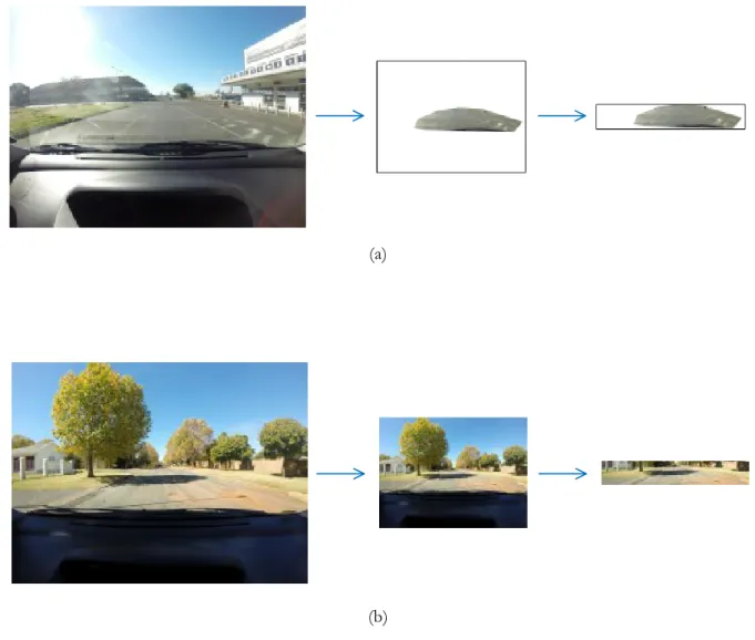
2.3.2 HISTOGRAM OF ORIENTED GRADIENTS

A basic diagram illustrating the extraction of HOG feature descriptors is shown in Figure 2.3.3. The first step is optional and comprises the normalisation of the gamma and colour of the image, and is introduced to compensate for a variation in lighting conditions. Gamma is a measure for the relationship between a pixel’s value and its luminance [40]. The normalisation is achieved by either determining the square root or log of the image intensity per channel [41].

Figure 2.3.3 HOG feature descriptor extraction [35]. The figure illustrates the steps required to determine the feature vector for detection. The first step is optional and will normalise the gamma of the image. Thereafter the gradients are computed per pixel. The gradients have both a magnitude and direction which can be used to obtain a histogram of orientations by sorting the magnitudes into bins based on their direction. Several cells are grouped together to form a block over which normalisation will take place. Lastly, the HOG of each window is placed in a feature vector and can be used for detection purposes.

In the second step the gradients within the image is computed (see Section 2.2.3). To determine the particular magnitude and direction of the gradient change, equations (2.2-4) and (2.2-5) are applied. From the third step onwards, to compute the HOG feature descriptor, it is necessary to divide the image into cells and blocks where the dimensions (width and height) of these components are specific to the object being detected. In the third step, a histogram of orientation is created per cell. The histogram is created by firstly deciding how many bins there should be in the histogram and what the maximum allowed orientation of the gradients are. For

(35)

22

example, if there are 9 bins, and the maximum allowed orientation of the vectors are chosen to be 180 degrees, the bins will be divided into 20 degree intervals (0 - 20 degrees, 20 - 40 degrees … 160 - 180 degrees). Then the magnitude of each of the vectors are added to the orientation bin to which the vector belongs to form a histogram. This process is done per cell and the number of bins and the maximum allowed orientation are kept constant.

The algorithm is made more robust in terms of lighting variations by combining several cells into a block and normalising over the block. Each block is then placed into a feature vector which can then be used as an input to an algorithm (such as a machine learning algorithm) to detect objects. The feature vector is also referred to as the HOG descriptor and its length can be calculated as in equation (2.3-1) [42].

HOG descriptor length = #Blocks * #CellsPerBlock * #BinsPerCell (2.3-2)

2.4 MACHINE LEARNING

2.4.1 INTRODUCTION

The point of applying machine learning to a problem is to develop a function that is able to take the input training data and create a model that can generalise well enough with respect to the data that it can provide accurate predictions on new data. If there is a wide variety in the data per class and not many similarities, it becomes difficult for the classifier to build a model that generalises satisfactorily [43]. Figure 2.4.1 illustrates the various types of fitting that can occur when training a two-class classifier. Figure 2.4.1.a and Figure 2.4.1.c both indicate model behaviour that is unwanted and is referred to as underfitting and overfitting, respectively. Note that when underfitting occurs, the model underestimates the data and more data is misclassified to the wrong class. When a model overfits, it fits the training data precisely but usually underperforms on test data as the model does not generalise enough. The most desired fitting for the data is shown in Figure 2.4.1.b which shows a good generalisation of the data without the model being too complex. There are a large number of options available when choosing a machine learning algorithm such as cascade classifiers [14, 32], SVMs (Support Vector Machines) [44] and ANNs (Artificial Neural Networks) that consist of MLP (Multi-Layer Perceptrons) [45].

(36)

23

Two different classifiers were selected in this thesis namely, a cascade classifier and a SVM (Support Vector Machine) which are discussed in this section. Thereafter, relevant important theory w.r.t. the classifiers as applied in this thesis is presented.

2.4.2 CASCADE CLASSIFIER

2.4.2.1 STANDARD CASCADE CLASSIFIER OPERATION

Cascade classifiers use several stages to classify data [14, 32]. The general structure of a cascade classifier is given in Figure 2.4.2. There are several stages directly connected in this structure. An input sample that needs to be classified is presented to the first stage which will either conclude that it is a negative sample and discard it or it will conclude that the sample might be a positive sample and, therefore, further testing of the sample is needed by sending the sample to the more advanced stages further down the structure in the cascade. The particular feature type (such as LBP) used during the training phase of the classifier, is also used to perform mathematical operations on the input sample. During training, different mathematical operations were executed for each stage of the classifier and yielded in certain thresholds for each stage. Therefore, a positive samples needs to fall within each of the trained thresholds for each stage in order to be classified as a positive sample. If at any point, any stage concludes that the input sample is a negative sample (by falling outside the particular threshold levels for a stage), it is labelled as a negative sample and the sample is not investigated further.

In unbalanced systems where there are more negative than positive samples, the probability of a sample being negative is much higher than the occurrence of a positive sample. For these

(a) (b) (c)

Figure 2.4.1 Graphs to show underfitting (a), good fit (b) and overfitting (c). The graphs indicate the result when a two-class two-classifier is required. With underfitting, it is clear that a large portion of the data of one of the two-classes (blue plusses)

(37)

24

types of systems, it is advantageous to use cascade classifiers as it is rarely necessary to perform the necessary calculations required for all of the stages for each sample which leads to a faster run-time. Stage 1 Positive classification Negative classification Stage 2 Stage N Negative classification Negative classification Positive classification

Figure 2.4.2 Cascade classifier working. Several stages are connected together where the positive classification of the previous stage is fed into the input of the next stage. If at any point, a stage classifies the input sample as negative, the sample is labelled as negative and the process exits. A true positive sample must be classified as positive by each of the stages in order to be classified correctly.

In [32], each of the stages consists of a single weak classifier. A weak classifier is a classifier that performs poorly on its own but is slightly better than randomly guessing Weak classifiers are

(38)

25

by definition not good enough to be used on their own, however, by combining them in a cascade manner, it is possible to create a very good classifier, which is discussed in the next section namely, boosting.

2.4.2.2 BOOSTING

The term boosting was first postulated in [46] which posed the question, whether using a number of weak learners/classifiers together could result in a stronger classifier with better accuracy. Boosting can be applied to cascade classifiers to improve their performance [32]. With boosting there are a series of iterations of the algorithm that takes place [47]. These iterations are used to determine the particular weight of a sample. It is required that all of the samples are labelled.

The boosting algorithm, was first introduced in [48] and is explained as follows: for all of the samples, the weight per sample start off as the same value. A decision stump then selects a sample. The feature value at that particular sample is then selected as the threshold value and, consequently, the weak learner classifies all of the samples below this threshold as positive and all of the samples above this as negative. Then, an update of the samples weights take place and the misclassified samples’ weights are increased. A new sample and threshold value is selected, based on the weights of all of the samples. The process continues for several iterations in a similar fashion. Lastly, all of the weak classifiers with their respective thresholds are aggregated together to form one classifier. Therefore, boosting effectively is a method for selecting the appropriate weak learner per iteration. This specific meta-algorithm that evaluates the samples based on their weights and updates the misclassified samples is known as AdaBoost [49].

2.4.3 SVM CLASSIFIER

SVMs are based on the theory of statistical learning and were first developed in [44, 50]. If it is assumed that the data is linearly separable, a linear support vector machine for a two-class problem can be used.

(39)

26

To explain the basic concept of a SVM, the case of the linear two-class SVM is considered in Figure 2.4.3. Given a plane such as the one in the figure and the example sample set in the plane, there exists a straight line that is equally spaced between the positive and negative samples which can be represented by the red dashed line. This line is known as either the decision boundary or the optimal hyperplane. The purpose of the SVM is to find the optimum placement of this hyperplane such that the margin (distance between the two red solid lines) is a maximum. The red line to the top of the optimal hyperplane is known as the positive boundary/hyperplane and is measured from the decision boundary to the closest positive samples that falls on the positive boundary. Similarly, there exists a negative boundary/hyperplane to the bottom of the decision boundary. The samples that fall on either the positive or negative boundaries, are known as support vectors. These support vectors are the only data points relevant to the calculation of the maximum hyperplane margin. w Example support vectors Margin

Figure 2.4.3 SVM hyperplane illustration. The feature set contains separable positive and negative samples. The decision boundary is represented with the red dashed line and a maximum margin (distance between the two red lines) is desired. Note that the decision boundary is equidistant from the positive and negative boundaries.

The derivation of the SVM is as follows: first, consider training data xi, where xi ∈ ℝ𝑚_and

has a label, yi ∈ {-1, +1}. In the figure, m = 2. Therefore the data are real elements in a 2-dimentional space. A positive sample is labelled as +1 and a negative sample is labelled as -1. The optimal hyperplane is expressed as:

(40)

27

w∙u + b = 0 (2.4-1) where b is an unknown bias constant and w is a weight vector that is perpendicular to the decision boundary.

The decision rule for a positive classification is equal to

w∙u + b ≥ 0 (2.4-2) and

w∙u + b < 0 (2.4-3)

for a negative classification. To solve the problem, we insert a positive and negative sample into the equation which leads to the following constraints:

w∙x++ b ≥ +1 when y

i = +1

w∙x-+ b ≤ -1 when y i = -1

(2.4-4)

Combining these equations with their respective labels leads to: yi(w∙x++ b) ≥ 1

(2.4-5) and

yi(w∙x- + b) ≥ 1, (2.4-6)

and finally a more general equation of

yi(w∙xi + b) - 1 ≥ 0 (2.4-7)

Now, to optimise the spacing of the decision boundaries, it is desired to have boundaries that are as wide as possible. The width of the boundaries can be determined by projecting the normalised vector w, onto the difference vector.

(41)

28 width = (x+ - x-)∙ w

‖w‖ (2.4-8)

From manipulating equations (2.4-4) and substituting the results into equation (2.4-8), the width of the margin is found to be 2/‖w‖. To determine the maximum width of the margin is mathematically equivalent to finding the minimum of the reciprocal of the margin. By mathematically manipulating and simplifying the maximum margin, equation (2.4-9) is found.

max_‖1

w‖ = min 1

2‖w‖2 (2.4-9)

The minimization is accomplished by applying Lagrangian multipliers (𝛼i) as the decision

vector w is the linear sum of some of the samples (the others equate to zero) [51]. Therefore, to solve the optimisation problem equation (2.4-10) is used.

L = 1

2‖w‖2 - ∑ 𝛼i

𝑙

𝑖=1

[yi(w∙xi + b) - 1] (2.4-10)

Minimising equation (2.4-10) over w by finding the partial Lagrangian derivatives and setting them to zero yields:

w = ∑ 𝛼i

𝑙

𝑖=1

yixi (2.4-11)

Similarly, by minimizing the same equation over b yields:

∑ 𝛼i

𝑙

𝑖=1

yi = 0 (2.4-12)

Substituting these equations back into the Lagrangian equation gives:

L = ∑ 𝛼i 𝑙 𝑖=1 - 1 2∑ ∑ 𝛼i𝛼j 𝑙 𝑗=1 yiyjxi∙xj 𝑙 𝑖=1 (2.4-13)

(42)

29

Finding the optimal parameter 𝛼o by applying the constraint of equation (2.4-12) and noting that all values for 𝛼 ≥ 0 will lead to the solution of the optimal hyperplane where bo is the value of b necessary for the optimal hyperplane:

∑ α_io

l

i=1

yixi + b_o = 0 (2.4-14)

The above process can be modified and repeated for the case where the data is not linearly separable and is known as soft margin classification [52].

From the SVM derivations on the previous pages, it was shown that the maximisation depends on only the vector dot product of the data vectors. The dot product between any two vectors has the property of 𝜙(xi) ⋅ 𝜙(xj) = K(xi,xj) where K(xi,xj) is a kernel function. A kernel

function can be used to perform the transformation in the vector space that separates the positive and negative samples/vectors. Example kernels [52] that are used with SVMs are:

 Linear: K(xi, xj) = xiTxj  Polynomial: K(xi, xj) = (γx_iTxj+ 𝑟)𝑑, 𝛾 > 0  RBF: K(xi, xj) = exp(-γ ‖x𝑖 −xj‖ 2 ), 𝛾 > 0  Sigmoid: K(x_i, x_j) = tanh(𝛾x_iT_x j+ 𝑟)

The choice of the kernel is a crucial factor in the performance of the SVM [53] and therefore careful consideration of the input data is necessary in order to select the most appropriate kernel.

2.4.4 SLIDING WINDOW AND IMAGE SCALING

A common approach to detect an object in an image is to apply a sliding window (usually much smaller than the original input image) to an image and scan the image for instances of the object. Another approach would be to detect any strong feature points in an image and try to match them to a trained model of the object. The latter is usually the case with SIFT and SURF feature extraction to perform image matching. Figure 2.4.4 illustrates the sliding window process where a square image of size 10 x 10 pixels is scanned with a 4 x 4 pixel sliding window (a.k.a.

(43)

30

detector window). The detector window starts in the top left corner and scan towards the right until it reaches the end of the image. It will then move one row down, and the process is the repeated. For each instance of the window in the image, the chosen features within the image is calculated and fed to the classifier for classification.

Frame Detector window

Figure 2.4.4 Sliding window functioning. An example input image of size 10 x 10 pixels is scanned with a detector window of 4 x 4 pixels. For each position of the detector window, features are calculated and used for detection purposes.

This process can only be used in instances where the object that needs to be detected is always of the same size. If the object size differs, it is necessary to either scale the image down by a factor repeatedly or to scale up the detector window by a factor repeatedly. This concept is demonstrated in Figure 2.4.5 which shows an example of how an image is repeatedly downsampled. In the figure the original image is scaled by 50% several times to produce the image pyramid. A sliding window approach will be applied to each of the scaled down images to detect the specific object in question. By using this approach, a scale-invariant classifier can be created to certain extent. This concept will be further discussed and demonstrated in Chapter 5.

There are some drawbacks to using a windowing function [55]. The first being that because the entire image is scanned for an object, any contextual information such as the usual region where the object is found is lost. In the case of potholes, for example, it is highly unlikely that a pothole will occur in the sky region of the image. The windowing function, will however, scan the entire image which increases the chance of detecting false positives. The second drawback of using a windowing function is the aspect ratio of the window is fixed which implies that the detected object must have the same fixed aspect ratio, otherwise, it cannot be detected. Potholes are not

(44)

31

fixed objects and have a high variation in appearance and size which makes them difficult to detect in general.

Figure 2.4.5 Image pyramid example with scale set to 50% [54]. The input image at the bottom of the pyramid is the original size and in this instance the image is downsampled by 50% for each step. Each image in the image pyramid is scanned with the detector window to determine if the object of interest is present or not.

2.5 EXISTING LITERATURE WITH RESPECT TO POTHOLE

DETECTION

2.5.1 DETECTION OF POTHOLES VIA VIBRATIONS

The simplest method for detecting potholes can be achieved by detecting the vibrations that a vehicle undoubtedly experience when it encounters a pothole. These vibrations can easily be measured by equipping the vehicle with an accelerometer [56]. This method for detecting potholes is only successful in conjunction with additional equipment that must log the position of the detected pothole via a GPS module. A form of communication (such as a GPRS module for example) is then necessary that can communicate this information to other vehicles/persons of interest before the pothole detections can be useful.

It is also possible to develop a pothole detector that only uses the accelerometer of a smartphone to detect potholes [57]. The on-board GPS and GPRS modules of the smartphone can then be used to upload the pothole detection to a central server which can distribute the

(45)

32

information accordingly. Smart phones have also become widely available and dropped substantially in price [58] making it a viable alternative option. However, from literature, it seemed that it has not yet been investigated how important the placement of the smart phone is inside the vehicle. It is possible that the built-in accelerometer would give a different reading if it was fixed to the vehicle, laying unfixed somewhere in the vehicle or when it is simply inside a passenger’s pants pocket or handbag. Further study is therefore needed in this area as this could create a major disadvantage if only smart phones are used.

In general, it is inexpensive to use vibrations to detect potholes and the solution would be even less expensive if it is assumed that most users already own a smart phone with accelerometer/GPS capabilities and it is only necessary to develop a cell phone software application. In [57], the average detector accuracy for events such as large potholes, small potholes, pothole clusters, gaps and drain pits is reported as 92% at best. Note, however, that by using this method, it is impossible to distinguish between the vibrations created by hitting a pothole or a drain pit.

Using only the measurements by an accelerometer it is clear that this method has an obvious downfall namely, for every pothole detected at least one vehicle must hit it. This is not an ideal situation as it is a very real possibility that the initial vehicle that detected the pothole sustained unwanted damage. Instinctively, a driver could also be inclined to swerve and try to avoid the pothole, which could minimize the new pothole detections in the system. It can also become a very complicated situation to distinguish between a pothole and the slamming of a door or encountering speed bumps [57].

2.5.2 VISUAL APPROACH

From analysing the literature it was found that using some type of visual approach that incorporates the use of at least one camera was the most popular choice for pothole detection. A visual approach is suitable, because generally, a pothole will look different in appearance when compared to the rest of the road/background to an observer. Visual cues are the only sensory input needed for a human to detect potholes with an extremely high accuracy rate when the human is giving their full attention to this task provided that the lighting conditions are reasonable. The complex task of visual object detection is relatively easy for humans compared to how difficult it is to teach a computer to “see”. For a child it is very easy, for example, to identify and classify a