Faisal Maqbool Zahid
Ordinal Ridge Regression with Categorical
Predictors
Technical Report Number 101, 2011
Department of Statistics
University of Munich
Ordinal Ridge Regression with Categorical Predictors
Faisal Maqbool Zahida,∗aLudwig-Maximilians-University Munich, Ludwigstrasse 33, D-80539 Munich, Germany.
Abstract
In multi-category response models categories are often ordered. In case of ordinal response models, the usual like-lihood approach becomes unstable with ill-conditioned predictor space or when the number of parameters to be es-timated is large relative to the sample size. The likelihood estimates do not exist when the number of observations is less than the number of parameters. The same problem arises if constraint on the order of intercept values is not met during the iterative procedure. Proportional odds models are most commonly used for ordinal responses. In this paper penalized likelihood with quadratic penalty is used to address these issues with a special focus on proportional odds models. To avoid large differences between two parameter values corresponding to the consecutive categories of an ordinal predictor, the differences between the parameters of two adjacent categories should be penalized. The considered penalized likelihood function penalizes the parameter estimates or differences between the parameters esti-mates according to the type of predictors. Mean squared error for parameter estiesti-mates, deviance of fitted probabilities and prediction error for ridge regression are compared with usual likelihood estimates in a simulation study and an application.
Key words: Likelihood estimation, Logistic regression, Non-proportional odds model, Partial proportional odds model, Penalization, Proportional odds model, Ridge regression.
1. Introduction
In regression analysis, maximum likelihood estimation is a common approach to compute the parameter estimates in categorical response models. But this approach fails if we have to estimate the parameters which are large in number relative to the sample size. In other words for a small ratio of sample size to the number of parameters (also forp>n
case) usual likelihood approach does not lead to a unique solution. The analyst faces the same problem for the data set with high correlation among the covariates and/or if there is a complete separation among the categories of the response variable. An alternative to the usual likelihood approach is to use penalized likelihood function. Penalization
∗Corresponding author. Tel.:++49 89 2180 6408; fax.:++49 89 2180 5040.
Email addresses:[email protected](Faisal Maqbool Zahid)
techniques combine log-likelihood function with a penalty term which measures the smoothness of the fit. In recent years several penalization techniques with different types of penalties have been proposed. The main objective of using penalized log-likelihood is to obtain unique estimates of the parameters, better prediction with a good compromise between bias and variance, and/or to have a sparse model for clear and easy interpretation of the parameter estimates. Ridge regression is the most familiar penalization approach in the literature. In the context of linear models much literature is available for ridge regression. Schaefer et al. (1984) and Schaefer (1986) discussed the ridge penalty for logistic regression with binary response. An extension of ridge regression for GLM type models is considered by Nyquist (1991). LeCessie and Houwelingen (1992) discussed different ways to select the ridge penalty and also for computing prediction error in case of logistic ridge regression. In the literature univariate GLM’s are more focused than the multivariate GLM. Zhu and Hastie (2004) used penalized logistic regression with quadratic penalty as an alternative to the support vector machine (SVM) for microarray cancer diagnostic problems. Zahid and Tutz (2009) used ridge penalty to get penalized estimates for logistic regression with multi-category (unordered) responses, which are independent of choice of the reference category. Ridge regression shrinks the parameter estimates to zero but none of them is exactly zero. As a result we do not have a parsimonious model but a model with all predictors. Another penalization approach called Lasso was proposed by Tibshirani (1996). Lasso technique not only shrinks the parameter estimates to zero but also serves as subset selection by setting some of the estimates exactly to zero. The lasso approach for multinomial logit models was considered by Friedman et al. (2010). In many applications multi-category responses are ordered. According to our knowledge penalization has not been addressed for ordered category response models. For ordinal responses there were several models discussed in the literature (see McCullagh (1980), Ananth and Kleinbaum (1997) and Agresti (1999)). However the proportional odds model (also known as cumulative logit models) is the most most popular among all other models for ordered category responses. Unlike multinomial logit models the proportional odds model (POM) has simple form in the sense that it has so-called global parameter estimates which are not category specific. But still in the case of large number of covariates maximum likelihood estimates may not exist. To resolve this problem we are using penalized log-likelihood with quadratic penalty to compute the estimates in proportional odds models. If the response variableY haskordered categories as
1, . . . ,k,the general form of the cumulative logit model is given by
loghP(Y ≤r|x)
P(Y >r|x) i
=γ0r−xTγγγr, r=1, . . . ,q=k−1. (1)
The vectorγγγTr = (γ1r, . . . , γpr) represents the category specific parameters. The simple form of proportional odds models with identical parameters for each category is given by
loghP(Y≤r|x)
P(Y>r|x) i
=γ0r−xTγγγ, r=1, . . . ,q=k−1. (2)
Here the so-called global parameters vectorγγγT =(γ1, . . . , γp) does not depend on the category. The ordered response Ycan be viewed as a categorized version of an unobservable latent variableZasY =r ⇔ γ0,r−1 <Z≤γ0rforr=
1, . . . ,k, where−∞ = γ00 < γ01 < . . . < γ0k = ∞define the category boundaries on the unobservable latent
continuum. The simple form of proportional odds model in (2) can be viewed as a univariate regression model for the latent variable with simple interpretation of parameters. The intercepts{γ0r}are different for each cummulative logit and must satisfy the stochastic orderingγ01 < . . . < γ0q to have positive probabilities. Also the negative sign in (1) and (2) ensures that the probability is increasing for large values ofxTγγγwith increasingr.
In the following text penalized estimates are computed using the penalized log-likelihood based on quadratic penalty for the simple form of the proportional odds models given in (2). In Section 2 penalized likelihood is discussed with some computational issues. The penalization with non-proportional odds models (NPOM) and partial proportional odds models (PPOM) is also described in this section. Empirical results of ordinal ridge regression are compared with usual ML estimates in Section 3. The ordinal ridge regression is fitted and compared with MLE using a real data in Section 4. The need of using penalized likelihood is also indicated in this section by drawing two small random samples of sizen =30 andn =50 from the considered real data where usual MLE is not existing. Some final and concluding remarks are given in Section 5.
2. Penalization and Computational Issues
For the proportional odds model given in (2), letφir(x) denote the cumulative probability for the occurrence of response
levels up to and includingrth level with a given covariate vectorxigiven as
φir(x)=P(Yi≤r|xi)=F(ηir) r=1, . . . ,q=k−1,
whereFis a strictly monotone distribution function. The model with homogeneous effects has the predictor
ηir=γ0r+xTiγγγ. (3)
In the context of multivariate generalized linear models, the simple proportional odds model can be given as
π π
πi=h(Xiβββ) or g(πππi)=Xiβββ,
whereπππTi =(πi1, . . . , πiq) with componentsπir=P(Yi=r|xi) andg=(g1, . . . ,gk−1) is a logit link type function given
by gr(πππi)=log log φir 1−φir −log φi,r−1 1−φi,r−1 . (4) Forp∗ = p+q,Xi = [Iq ×q,1q×1⊗xTi] is aq×p∗matrix andβββT =(γγγT0, γγγT) =(γ01, . . . , γ0q, γ1, . . . , γp) is ap∗×1
vector. The complete design matrix of ordernq×p∗is given asXT =[X
1, . . . ,Xn].For further details see McCullagh
and Nelder (1989) and Fahrmeir and Tutz (2001).
The predictor space may contain some categorical predictors with more than one parameters associated with it. Let we haveKj parameters associated with predictorxj.So for a binary or continuous covariate we have Kj = 1 and
if covariate is categorical thenKj > 1 depending upon the number of categories of the predictorxj.The penalized log-likelihood with quadratic penalty is given as
lp(βββ)=l(βββ)−λ2J(βββ), (5)
wherel(βββ) is the usual log-likelihood function given by
l(βββ)= n X i=1 k X r=1 yirlog(πir), (6)
andλis a tuning parameter. The penalty termJ(βββ) can be given as
J(βββ)=βββTPβββ. (7)
The definition of penalty matrixPdepends on how we perform penalization with different types of predictors. If we have some ordinal predictors in the predictor space, penalization should be applied in such a way that ordinal covari-ates can be distinguished from the other covaricovari-ates by considering the order of the categories. In penalization, it is common practice to penalize the parameter estimates but with ordinal predictors rather than estimates, difference be-tween the parameters estimates of adjacent categories should be penalized (see Gertheiss and Tutz (2009)). Penalizing such differences will cause a smoothed version of the parameter estimates by avoiding the large difference among the estimates associated with the dummies of the ordinal predictors. Let the predictorxjis ordinal withKj+1 categories and first category is treated as reference category. Ifγγγj denotes the parameter vector forKj parameters/dummies associated with ordinal predictorxj, the penalty term for penalizing the differences between parameters of adjacent categories takes the form as
J(γγγj)= K+1
X l=2
(γjl−γj−1,l)2=γγγTj ΩΩΩjγγγj, withΩΩΩj=UTjUj,for aKj×KjmatrixUjgiven by
Uj= 1 0 · · · 0 −1 1 . .. ... 0 −1 1 . .. ... .. . . .. ... ... 0 0 · · · 0 −1 1 .
If the predictor is not ordinal then the penalty term for predictorxjis given by
J(γγγj)= K+1
X l=2
γ2jl=γγγTj Ijγγγj,
whereIjis aKj×Kj identity matrix. For the predictor space with all types of predictors (i.e., binary/continuous, nominal and ordinal predictors), the penalty matrixPgiven in (7) is given by
P=diag(0q×q,P1, . . . ,Pp). (8)
Here0q×q is a zero matrix with zeros for the category specific intercept terms which are not penalized. If the jth predictor is ordinal then (Kj×Kj)−submatrixPjassumes the valueΩΩΩjotherwisePj=Ij.
The penalized log-likelihood function given in (5) can be written as
lp(βββ)= n X i=1 li(βββ)−λ2 p X j=1 βββTjPβββj Score functionsp(βββ) for the penalized log-likelihood is given by
sp(βββ) = n X
i=1
XT
iDi(βββ)ΣΣΣ−i1(βββ)[yi−h(ηηηi)]−λPβββ
= XTD(βββ)ΣΣΣ−1(βββ)[y−h(ηηη)]−λPβββ (9) whereDi(βββ) = ∂h(ηηηi)
∂ηηη is derivative of h(ηηη) evaluated atηηηi = Xiβββ,ΣΣΣi(βββ) = cov(yi) is the covariance matrix of ith observation ofygiven parameter vectorβββandWi(βββ)=Di(βββ)ΣΣΣi−1DTi(βββ).yandh(ηηη) are given byyT =(yT
1, . . . ,yTn) and
h(ηηη)T =(h(ηηη1)T, . . . ,h(ηηηn)T).The matrices have block diagonal formΣΣΣ(βββ) =diag(ΣΣΣ−i1(βββ)), D(βββ) =diag(Di(βββ)) and W(βββ)=diag(Wi(βββ)).By equating the score function to zero we obtain the estimation equations as
XTD(βββ)ΣΣΣ−1(βββ)[y−h(ηηη)]−λPβββ=0,
whereβββisp∗×1 parameter vector forp∗=q+Pp
j=1KjandPis ap∗×p∗matrix given in (8). Fisher scoring iteration
yields ˆ βββ(k+1) = βββˆ(k)+ XT Wβββˆ(k)X+λP−1s p βββˆ(k).
If ˆβββare penalized estimates for the true parameterβββ,the covariance matrix can be approximated by cov(ˆβββ) =
XTWβββˆX+λP−1XT WβββˆXXTWβββˆX+λP−1.
Generalized cross-validation (GCV) criterion is used to find the optimal value of ridge penaltyλ.In the generalized linear models (GLM) environment we are using likelihood-based criterion deviance for GCV instead of squared distances ofyi.andπi..Deviance based generalized cross-validation is given by
GCV=−2.
Pn
i=1(lλ(ˆπππi)−li(yi))
(1−tr(H(λ))/n)2 , (10)
where the the hat matrixHis given as
H=WT/2X
XT WβββˆX+λP−1XTW1/2.
In this text we are using penalization to address the problems with likelihood estimation for proportional odds models which are commonly used with ordered response categories. But some problems may become more critical when we are dealing with non-proportional odds models (NPOM) given in (1) with category specific parameters or partial proportional odds model (PPOM) given by
ηir=γ0r+xTiGγγγG+xTiLγγγLr r=1, . . . ,q, (11)
where some of the parameters have global effectγγγGand others have local/category specific effectγγγLr.In both of these types of models we have to estimate more parameters than in the corresponding proportional odds model. In case of non-proportional or partial proportional odds models, penalization can be implemented in the same way as for POM. The only difference is that the structure of design matrix will be changed according to the model. In case of proportional odds model the design matrix forith observation is aq×p∗matrixXi=[Iq×q,1q×1⊗xT
i] withp∗=p+q, as discussed above. For non-proportional odds model the design matrix assumes the same structure as for multinomial logit models and for theith observation is given asXi =[Iq×q,Iq×q⊗xTi].For partial proportional odds models the design matrix can be written asXi = [Iq×q,1q×1⊗xGiT,Iq×q⊗xTLi] wherexTGiis a vector associated with predictors having global effect andxT
Liis a vector of observations for those predictors having local i.e., category specific effect. The parameter vector associated with POM, NPOM and PPOM are given byβββT =(γγγT0, γγγT)=(γ01, . . . , γ0q, γ1, . . . , γp), βββT =(γγγT0, γγγT1, . . . , γγγTq) andβββT =(γγγT0, γγγTG, γγγTL1, . . . , γγγTLq) respectively. In case of NPOM and PPOM, the penalty matrixP has a higher dimension than the proportional odds models and can be formulated according to the structure of design matrix based on the desired model to fit.
3. Simulation Study
The effectiveness of ridge regression is discussed in this section using simulated data. For a sample of sizenpredictor space contains continuous covariates (denoted byC), binary covariates (denoted byB), nominal covariates (denoted byNK+1) and/or ordinal covariates (denoted byOK+1) with K+1 categories. The continuous covariates are drawn
from a p-dimensional centered multivariate normal distribution with covariance between two covariatesxj andxk beingρ|j−k|.Four values ofρ=0.0,0.3,0.7 and 0.9 are used. To study the problems with existence of usual MLE, we consider proportional odds models withk=3 andk=5 response categories for each setting of predictor space given in Table 1. The true values used for the intercept terms are (−0.3,0.8) and (−0.8,−0.3,0.3,0.8) fork=3 andk=5 respectively. The true values for global parameters are obtained as (−1)jexp(−2(j−1)/20) for j=1, . . . ,Pp
j=1Kj.A
multiplicative factorcsnrforβββT =(γγγT0, γγγ) is chosen so that the signal-to-noise ratio is 1.
T able 1: Comparison of ridge estimates and maximum lik elihood estimates in terms of MSE( ˆβββ), de viance( ˆ πππ )and mean prediction error (MPE). Results of simulation study for setting 1 ( C = 10), and setting 2 ( C = B = 5 , N3 = N4 = O3 = O4 = 1) . k = 3 response cate gories k = 5 response cate gories MLEMLEMLE RidgeRidgeRidge MLEMLEMLE RidgeRidgeRidge Predictors ρ n MSE( ˆβββ) de v( ˆπππ) MPE MSE( ˆβββ) de v( ˆπππ) MPE S 0 MSE( ˆβββ) de v( ˆπππ) MPE MSE( ˆβββ) de v( ˆπππ) MPE S 0 Setting 1 0 . 0 30 180 . 1517 13 . 6873 812 . 7266 7 . 0702 14 . 3484 311 . 5942 581 226 . 4500 17 . 8471 1249 . 4654 11 . 0557 18 . 7363 442 . 4797 2058 0 . 3 30 291 . 1177 12 . 0787 1798 . 7247 9 . 2962 13 . 3363 370 . 9956 500 691 . 2087 14 . 4727 2642 . 9824 14 . 2578 16 . 4372 492 . 4584 1129 0 . 7 30 343 . 8420 13 . 6453 941 . 6172 11 . 4605 14 . 8170 292 . 5661 535 1455 . 5374 14 . 5094 3095 . 8244 15 . 2049 17 . 3496 351 . 6358 1045 0 . 9 30 421 . 3659 13 . 1603 883 . 5063 15 . 3219 14 . 9178 179 . 8458 366 714 . 1525 18 . 9570 1690 . 2692 16 . 9764 20 . 7584 278 . 5656 2012 0 . 0 50 14 . 7393 21 . 3033 272 . 5190 4 . 4841 21 . 6354 177 . 3077 34 12 . 7195 30 . 8484 301 . 3216 4 . 5850 31 . 0682 206 . 5610 104 0 . 3 50 14 . 2448 24 . 1852 257 . 8009 3 . 9573 24 . 6463 168 . 2815 191 12 . 7935 29 . 9773 368 . 6335 5 . 6757 30 . 2297 258 . 8844 71 0 . 7 50 19 . 2019 22 . 5475 206 . 5454 5 . 9453 23 . 0144 122 . 8994 55 22 . 1063 28 . 8023 299 . 0853 8 . 7088 29 . 1385 186 . 4700 91 0 . 9 50 43 . 6299 22 . 4499 349 . 7897 11 . 8912 23 . 4773 171 . 2196 28 37 . 6087 30 . 7496 241 . 6781 11 . 6172 31 . 6667 134 . 3995 225 0 . 0 100 3 . 7835 47 . 4030 97 . 2800 2 . 3563 47 . 5027 82 . 8500 0 3 . 8077 64 . 8215 103 . 6088 2 . 2826 64 . 9884 88 . 0231 5 0 . 3 100 2 . 7517 48 . 1384 96 . 9192 2 . 0136 48 . 2122 86 . 0813 0 4 . 5805 61 . 0400 118 . 8080 3 . 2509 61 . 1268 102 . 3104 1 0 . 7 100 7 . 1912 46 . 4471 111 . 7852 4 . 2880 46 . 6742 89 . 7360 0 5 . 0293 64 . 5797 100 . 7663 3 . 3961 64 . 7084 84 . 9762 6 0 . 9 100 26 . 2696 41 . 8972 74 . 2318 10 . 9573 44 . 0150 51 . 0959 0 17 . 4760 60 . 7705 89 . 1357 7 . 2828 61 . 6250 64 . 1689 7 Setting 2 0 . 0 30 − − − 43 . 7581 6 . 3059 843 . 4785 − − − − 102 . 7840 7 . 6073 1073 . 9108 − 0 . 3 30 − − − 66 . 1659 5 . 2765 833 . 6123 − − − − 60 . 5190 10 . 4094 803 . 4053 − 0 . 7 30 − − − 83 . 3968 6 . 3192 618 . 4994 − − − − 92 . 9740 9 . 6020 601 . 8936 − 0 . 9 30 − − − 80 . 9918 4 . 9503 529 . 5153 − − − − 54 . 8040 11 . 2600 444 . 5055 − 0 . 0 50 1115 . 9632 21 . 1014 1579 . 6180 24 . 0194 22 . 9401 372 . 7722 3729 155 . 9596 33 . 9577 565 . 9361 24 . 2283 35 . 8264 252 . 0067 117090 0 . 3 50 606 . 7988 21 . 6298 977 . 6950 35 . 5278 22 . 5852 336 . 4792 3202 191 . 1933 31 . 5447 730 . 8627 35 . 8602 33 . 2564 288 . 3899 222630 0 . 7 50 115 . 9206 23 . 6653 786 . 0302 24 . 6058 25 . 3760 330 . 2098 11037 89 . 1062 33 . 0967 622 . 6985 32 . 5620 34 . 8354 328 . 4705 177954 0 . 9 50 276 . 7447 23 . 0867 980 . 9997 34 . 9713 25 . 3711 292 . 1317 13631 750 . 8599 31 . 0706 1078 . 0603 41 . 9371 33 . 0903 325 . 7565 108679 0 . 0 100 48 . 8578 41 . 6153 265 . 6948 22 . 0897 42 . 4914 175 . 4264 121 54 . 2255 61 . 3517 208 . 9794 22 . 7296 62 . 2579 145 . 6910 251 0 . 3 100 36 . 9882 43 . 8864 267 . 5244 19 . 2712 44 . 4978 184 . 9282 46 36 . 1564 61 . 4025 249 . 0228 19 . 4544 62 . 1226 173 . 3752 221 0 . 7 100 47 . 7568 43 . 4548 281 . 4263 17 . 4481 44 . 6789 168 . 8737 24 41 . 0952 61 . 5909 248 . 1124 20 . 4104 62 . 4173 165 . 9631 183 0 . 9 100 41 . 9465 47 . 0938 242 . 1356 17 . 8432 48 . 1940 151 . 0515 44 75 . 0072 41 . 0731 255 . 6754 35 . 6351 42 . 5402 150 . 1283 1562984 7
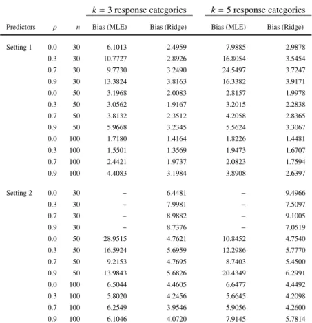
Table2: Comparison of Bias in ridge estimates and maximum likelihood estimates. Results of simulation study for setting
1 (C=10), and setting 2 (C=B=5, N3=N4=O3=O4=1).
k=3 response categories k=5 response categories Predictors ρ n Bias (MLE) Bias (Ridge) Bias (MLE) Bias (Ridge)
Setting 1 0.0 30 6.1013 2.4959 7.9885 2.9878 0.3 30 10.7727 2.8926 16.8054 3.5454 0.7 30 9.7730 3.2490 24.5497 3.7247 0.9 30 13.3824 3.8163 16.3382 3.9171 0.0 50 3.1968 2.0083 2.8157 1.9978 0.3 50 3.0562 1.9167 3.2015 2.2838 0.7 50 3.8132 2.3512 4.2058 2.8365 0.9 50 5.9668 3.2345 5.5624 3.3067 0.0 100 1.7180 1.4164 1.8226 1.4481 0.3 100 1.5501 1.3569 1.9473 1.6707 0.7 100 2.4421 1.9737 2.0823 1.7594 0.9 100 4.4083 3.1984 3.8908 2.6397 Setting 2 0.0 30 − 6.4481 − 9.4966 0.3 30 − 7.9981 − 7.5097 0.7 30 − 8.9882 − 9.1005 0.9 30 − 8.7376 − 7.0519 0.0 50 28.9515 4.7621 10.8452 4.7540 0.3 50 16.5924 5.6959 12.2986 5.7770 0.7 50 9.2153 4.7695 8.7403 5.4500 0.9 50 13.9843 5.6826 20.4349 6.2991 0.0 100 6.5044 4.4605 6.6477 4.4492 0.3 100 5.8020 4.2456 5.6645 4.2098 0.7 100 6.2549 3.9546 5.9056 4.2600 0.9 100 6.1046 4.0720 7.9145 5.7814
For each setting mentioned in Table 1 with different number and type of covariates,S =50 samples of sizenare used in the study. To compare the results of ridge estimates with likelihood estimates we consider only those samples for which ML estimates exist. In order to obtainS =50 samples,S0samples are ignored because ML estimates with their standard errors are not existing for these samples usingpolrfunction of libraryMASSin statistical language R 2.10.0.
In Table 1, the columns with titleS0showing the number of samples for which ML estimates did not exist, highlights
the need of a penalization technique. The results of Table 1 show that value ofS0 is increasing with increasing
number of predictors drawn from different distributions. This problem becomes even more severe withk=5 response categories. For sample sizen = 30,we cannot generate 50 samples for which MLE is existing in setting 2 and in
setting 1 although estimates are presented but they have quite large standard errors (not shown here). Although ML estimates become more stable for independent predictors or in case of moderate correlation among predictors with increasing sample size, however they are deteriorated in case of high multicollinearity. The ridge regression may be the best choice to obtain stable estimates of parameters for all predictors in the model when usual MLE is not existing or deteriorated because of ill-conditioned predictor space. In Table 1, ML estimates are computed usingpolrfunction of statistical environment/language R 2.10.0. Ridge estimates are compared with likelihood estimates in terms of
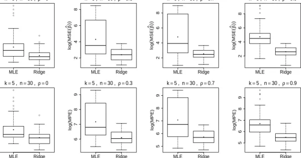
● ● ● ● ● ● MLE Ridge 2 4 6 8 log ( MSE ( β ^)) ● ● k=5 , n=30 , ρ =0 MLE Ridge 2 4 6 8 log ( MSE ( β ^)) ● ● k=5 , n=30 , ρ =0.3 MLE Ridge 2 4 6 8 log ( MSE ( β ^)) ● ● k=5 , n=30 , ρ =0.7 ● ● ● ● MLE Ridge 2 4 6 8 log ( MSE ( β ^)) ● ● k=5 , n=30 , ρ =0.9 ● ● ● ● ● ● MLE Ridge 5 6 7 8 9 log(MPE) ● ● k=5 , n=30 , ρ =0 MLE Ridge 6 7 8 9 log(MPE) ● ● k=5 , n=30 , ρ =0.3 MLE Ridge 5 6 7 8 9 log(MPE) ● ● k=5 , n=30 , ρ =0.7 ● ● ● ● MLE Ridge 5 6 7 8 9 log(MPE) ● ● k=5 , n=30 , ρ =0.9
Figure1: Illustration of simulation study for ten predictors drawn from multivariate normal distribution fork=5 response
categories: Box plots for comparing ridge estimates with ML estimates in terms of log(MSE(ˆβββ)) (top panel) and log values of Mean Prediction Error i.e., log(MPE) (bottom panel). The solid circles within the boxes represent the mean of the observations for which box plots are drawn.
mean squared error (MSE) of ˆβββ,deviance of the fitted probabilities and mean prediction error (MPE). In all settings we use samples of sizen for the training data and then a sample of sizentest = 1000 is generated for comparing the prediction performance of ridge estimates with likelihood estimates. The results of Table 1 show that ridge is performing better than MLE as is expected. In case of ten normally distributed covariates, ML estimates have very large standard errors forn =30.In the simulation setting 2 considered with categorical predictors there are twenty
parameters to be estimated (other than intercept terms). Here the situation goes more worse with MLE and we have to leave a large number of samples (especially withk =5 response categories) because of problems with existence of estimates. Even we could not get enough samples withn=30 for which likelihood estimates with their standard errors exist. So for setting 2 withn=30 only the results of ridge regression are given in Table 1. The ridge estimates do exist in all considered situations even when the likelihood estimates do not exist. For comparing ridge estimates with ML estimates, mean squared error is computed as 1
S Ps (ˆβββmethods −βββtrue)T(ˆβββ
method
s −βββtrue) and the formula used to compute deviance of fit i.e., Dev(ˆπππ) is given byD=2.Pi=n1Pkj=1yi jlogyi j
ˆ πi j withyi jlog y i j ˆ πi j =0 foryi j =0.Mean prediction error based on 1000 test observations is computed as MPE= S1PsDs= S1Ps2.h Pni=1Pkj=1πtesti jslog
πtest i js ˆ πtesti js i .
In addition to MSE(ˆβββˆˆ) it is also important to observe the amount of bias in the parameter estimates. The mean length
of vectors of bias inS = 50 samples is computed for ridge and ML estimates as S1 Ps||βββˆmethods −βββtrue||.The mean values for lengths of bias vectors for MLE and ridge estimates is given in Table 2 for each setting of simulation study. The graphical representation of the results for more interesting cases with small samples fork=5 response categories
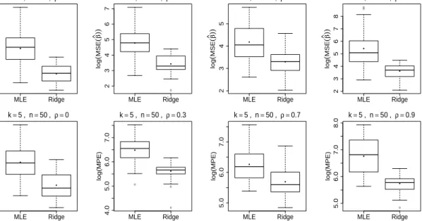
MLE Ridge 2 3 4 5 6 7 log ( MSE ( β ^)) ● ● k=5 , n=50 , ρ =0 ● MLE Ridge 2 3 4 5 6 7 log ( MSE ( β ^)) ● ● k=5 , n=50 , ρ =0.3 MLE Ridge 2 3 4 5 log ( MSE ( β ^)) ● ● k=5 , n=50 , ρ =0.7 ● ● MLE Ridge 2 3 4 5 6 7 8 log ( MSE ( β ^)) ● ● k=5 , n=50 , ρ =0.9 MLE Ridge 5.0 5.5 6.0 6.5 7.0 7.5 log(MPE) ● ● k=5 , n=50 , ρ =0 ● ● ● MLE Ridge 4.0 5.0 6.0 7.0 log(MPE) ● ● k=5 , n=50 , ρ =0.3 MLE Ridge 5.0 6.0 7.0 log(MPE) ● ● k=5 , n=50 , ρ =0.7 ● MLE Ridge 5.0 6.0 7.0 8.0 log(MPE) ● ● k=5 , n=50 , ρ =0.9
Figure2: Illustration of simulation study fork=5 response categories andC =B =5 andN3 =N4 =O3 =O4 =1
predictors in the predictor space: Box plots for comparing ridge regression estimates with MLE in terms of log(MSE(ˆβββ)) (top panel) and Mean Prediction Error i.e., log(MPE) (bottom panel). The solid circles within the boxes represent the mean of the observations for which box plots are drawn.
is given in Figure 1 and 2 with the help of box plots. The solid circles in each box represents the mean of the values for which box plot is drawn.
4. Application
In this section for computing and comparing the ridge estimates with ML estimates, we are considering the housing
data set from UCI repository (http://archive.ics.uci.edu/ml/datasets/Housing). The response variable
(MEDV) is about the median values of the owner-occupied houses in suburbs of Boston. For the analysis purpose, response variable which is measured in $1000’s is divided into four price categories as lower , lower middle, upper middle and high price category using the thresholds as MEDV< 10,10 ≤ MEDV < 25,25 ≤ MEDV < 40 and
MEDV ≥40.The predictors used to predict the price range of a house are: per capita crime rate by town (CRIM);
proportion of residential land zoned for lots over 25,000 sq.ft. (ZN); proportion of non-retail business acres per town (INDUS); Charles River dummy variable (CHAS=1 if tract bounds river; CHAS=0 otherwise); nitric oxides con-centration (NOX)(parts per 10 million); average number of rooms per dwelling (RM); proportion of owner-occupied units built prior to 1940 (AGE); weighted distances to five Boston employment centres (DIS); index of accessibility to radial highways (RAD); full-value property-tax rate per $10,000 (TAX); pupil-teacher ratio by town (PTRATIO); 1000(Bk−0.63)2 where Bk is the proportion of blacks by town (B) and % lower status of the population (LSTAT).
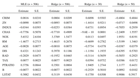
Although thepolrfunction of R provides the likelihood estimates of parameters but fails to produce standard errors of these estimates. So the usual ML estimates and corresponding standard errors are not computed withpolras in simu-lation study but ML estimates are computed forλ=0.For computing the ridge estimates, ridge penalty is decided on the basis of deviance based generalized cross-validation (GCV). The parameter estimates with their standard errors are given in Table 3 for the complete data set. The results of ridge regression are based on the optimal value of ridge penaltyλ=0.1.In order to check the existence of MLE in case of small samples, different random samples of size n =30 are drawn from the complete data set and likelihood estimates are not existing for any of the these samples. Similarly ML estimates are not existing for most of the random samples of sizen =50 drawn from total sample of sizen=506.However ridge estimates are existing for all such small samples. Two such small samples withn=30 andn=50 are considered for which MLE is not existing but ridge estimates do exist. Both of these data sets can be
accessed atwww.stat.uni-muenchen.de/∼zahid/samples ordinalRidge.txt. The parameter estimates and
their standard errors for ridge regression with these two samples are given in Table 3. The ridge estimates in both of these small samples are computed with optimal value of ridge penaltyλ=0.1.
Table3: MLE and ridge estimates with corresponding standard errors for complete housing data set (n=506) and ridge
estimates with their standard errors for random samples of sizen=30 andn=50 drawn from the complete data set. MLE (n=506) Ridge (n=506) Ridge (n=30) Ridge (n=50)
Estimate S.E. Estimate S.E. Estimate S.E. Estimate S.E.
CRIM 0.0816 0.0210 0.0804 0.0209 0.6898 0.9303 −0.4804 0.4044 ZN −0.0090 0.0075 −0.0093 0.0075 −1.4414 0.9211 −0.0717 0.0498 INDUS −0.0344 0.0393 −0.0253 0.0384 0.6731 0.8954 −0.7055 0.2939 CHAS −0.7756 0.5078 −0.7710 0.4909 −9.6E−10 0.0001 −2.2409 1.5557 NOX 5.6532 2.6104 3.3769 1.5477 0.0113 0.0497 1.9551 0.8191 RM −1.4677 0.2715 −1.4615 0.2678 −0.4699 0.2782 −3.5199 1.3463 AGE −0.0028 0.0077 −0.0010 0.0075 −0.5734 0.4378 −0.0387 0.0379 DIS 0.4321 0.1243 0.3970 0.1186 −1.1194 1.1935 −0.6395 0.5703 RAD −0.2029 0.0475 −0.1952 0.0465 −0.3114 0.5659 −0.5855 0.2925 TAX 0.0077 0.0025 0.0077 0.0025 0.0394 0.0752 0.0386 0.0172 PTRATIO 0.3756 0.0844 0.3501 0.0804 1.9405 1.2744 1.1177 0.4431 B −0.0077 0.0022 −0.0077 0.0022 −0.2529 0.5010 0.0092 0.0102 LSTAT 0.3082 0.0432 0.3119 0.0430 0.1750 0.8308 0.9086 0.3917
5. Concluding Remarks
Ridge regression provides stable estimates in logistic regression when maximum likelihood estimates are deteriorated because of ill-conditioned predictor space. Multicollinearity among the predictors causes an increase in the average length of likelihood estimates of parameter vector and inflates the standard errors of these estimates. Also when
sample size is small relative to the number of parameters, existing softwares for fitting proportional odds models may face the problems in computing the estimates and especially with computing standard errors of the estimates (e.g.,
polrfunction ofMASSpackage in R that we used in this text may provide the parameter estimates for some data sets but fails to produce the corresponding standard errors). Ifp∗ >nthe maximum likelihood estimates will not exist at
all. If stochastic ordering of estimates for the intercepts is disturbed during iterative process, it will lead to illogical values of the fitted probabilities. To address all of these issues, ridge regression is used in this paper for ordinal response models with a focus on proportional odds models. However for non-proportional odds models or partial proportional odds models the ridge regression can be used easily in the same way. The only difference is that we have to penalize more parameter estimates depending upon the model/design space under consideration as discussed in the end of Section 2. Since ridge penalty shrinks the parameters estimates to zero but does not perform variable selection, it is useful in case of limited number of predictors where the analysts are interested in fitting a model by keeping all the predictors in the model. With penalization, parameter estimates corresponding to the categorical predictors are penalized by considering whether it is a nominal or ordinal predictor. For ordinal predictors differences between the parameters estimates of successive categories should be small. In this paper, these differences are kept small by penalizing the differences between successive parameters estimates of ordinal predictors instead of penalizing the estimates themselves.
References
Agresti, A., 1999. Modelling ordered categorical data: Recent advances and future challenges. Statistics in Medicine 18, 2191–2207.
Ananth, C. V., Kleinbaum, D. G., 1997. Regression models for ordinal responses: A review of methods and applications. International Journal of Epidemiology 26, Number 6, 1323–1333.
Fahrmeir, L., Tutz, G., 2001. Multivariate Statistical Modelling based on Generalized Linear Models. second ed. Springer-Verlag NewYork, Inc. Friedman, J., Hastie, T., Tibshirani, R., 2010. Regularization paths for generalized linear models via coordinate descent. Jounal of Statistical
Software 33, Issue 1.
Gertheiss, J., Tutz, G., 2009. Penalized regression with ordinal predictors. International Statistical Review 77, 345–365. LeCessie, S., Houwelingen, V., 1992. Ridge estimators in logistic regression. Applied Statistics 41, 191–201.
McCullagh, P., 1980. Regression models for ordinal data. Journal of the Royal Statistical Society B 42, 109–142. McCullagh, P., Nelder, J., 1989. Generalized Linear Models. second ed. Chapman & Hall, NewYork.
Nyquist, H., 1991. Restricted estimation of generalized linear models. Journal of Applied Statistics 40, 133–141.
Schaefer, R., 1986. Alternative estimators in logistic regression when the data are collinear. Journal of Statistical Computation and Simulation 25, 75–91.
Schaefer, R., Roi, L., Wolfe, R., 1984. A ridge logistic estimator. Communications in Statistics: Theory and Methods 13, 99–113.
Tibshirani, R., 1996. Regression shrinkage and selection via lasso. Journal of the Royal Statistical Society B 58, 267–288.
Zahid, F. M., Tutz, G., 2009. Ridge estimation for multinomial logit models with symmetric side constraints. Technical Report No. 67. Institute of Statistics, Ludwig-Maximilians-University Munich, Germany.
Zhu, J., Hastie, T., 2004. Classification of gene microarrays by penalized logistic regression. Biostatistics 5, 427–443.