On Filtering in Markovian Term Structure Models
(an approximation approach)
Carl Chiarella
School of Finance and Economics, University of Technology Sydney
PO Box 123, Broadway NSW 2007, Australia
[email protected]
Sara Pasquali
Dipartimento di Matematica, Universit´
a degli Studi di Parma
85, Via M. D’Azeglio, I - 43100 Parma, Italy
[email protected]
Wolfgang J. Runggaldier
Dipartimento di Matematica Pura ed Applicata
Universit´
a di Padova, 7 Via Belzoni, I - 35131Padova, Italy
[email protected]
September 12, 2001
Abstract
We study a nonlinear filtering problem to estimate, on the basis of noisy observations of forward rates, the market price of interest rate risk as well as the parameters in a particular term structure model within the Heath-Jarrow-Morton family. An approximation approach is described for the actual computation of the filter.
Key words : Filter approximations, Heath-Jarrow-Morton model, market price of inter-est rate risk, Markovian representations, measure transformation, nonlinear filtering, term structure of interest rates.
MSC Classification : 90A09, 93E11, 60G35, 62F15, 62M05.
1
Introduction
The paper by Heath, Jarrow and Morton [14] (henceforth HJM) marked an important step in the development of models of the term structure of interest rates. The HJM model had been
presaged by the simpler (and less general) Ho-Lee [15] model. The HJM model distinguished itself from previous term structure models, which were essentially based conceptually on the approach of Vasicek [24], by providing a pricing framework that is consistent with the currently observed yield curve and whose major input is a function specifying the volatility of forward interest rates. To this extent it can be viewed as the complete analogue, in the world of stochastic interest rates, to the Black-Scholes model of the deterministic interest rate world that prices derivatives consistently with respect to the price of the underlying asset (of which the currently observed yield curve is the analogue) and requires as its major input the volatility of returns of the underlying asset (to which the forward rate volatility function is the analogue).
The challenges posed in implementing the HJM model arise from the fact that in its most general form the stochastic dynamics are non-Markovian in nature. As a result most implementations of the HJM model revolve around some procedure, and/or assumptions, that allow the stochastic dynamics to be re-expressed in Markovian form - usually by employing the “trick” of expanding the state-space.
As we have stated above the major input into the HJM model is the forward rate volatility function and indeed its specification will determine the nature of the stochastic dynamics and whether and how it then can be reduced to Markovian form.
In view of finite dimensional realizations of HJM models (for a general study see [6]), Chiarella and Kwon [8], [9] have shown that a broad, and important for applications, class of interest rate derivative models whose dynamics can be “Markovianised” can be obtained by assuming forward rate volatility functions that depend on a finite set of forward rates with given maturities as well as time to maturity.
An important practical problem faced in implementing such term structure models is the estimation of the parameters entering into the specification of the forward rate volatility function. In fact, one of the major aims of this paper is to show how this estimation problem can be approached within a filtering framework.
In section 2 we introduce our basic model that is a particular version of the HJM model set-up within the Chiarella-Kwon [8], [9] framework in which the volatility function depends on the instantaneous spot rate of interest (maturity of zero), one forward rate of fixed ma-turity and, time to mama-turity. Under the risk-neutral probability measure the stochastic dy-namics of the spot rate and of the fixed maturity forward rate are given by a two-dimensional Markovian stochastic differential equation system. However as our observations occur under the so-called historical probability measure, we need to introduce also the market price of interest rate risk (that connects the two probability measures). We assume that the market price of risk follows a mean reverting process and so, under the historical measure, we are left with a three-dimensional Markovian stochastic differential system. A truncation factor is furthermore added to the coefficients thereby guaranteeing existence and uniqueness of a strong solution that takes values in a compact set. Assuming that the information comes from noisy observations of the fixed-maturity forward rate, in this same section 2 we also formulate the filtering problem, whose solution leads to the estimation of the market price
of risk and of the unobserved instantaneous rates of interest and as well as of the parameters in the model.
The resulting filtering problem is highly nonlinear so that approximation methods have to be used for its solution. We shall describe a method, based on time discretization that, together with further approximations (quantization), leads to a discrete time approximating problem for which a filter of fixed finite dimension can be derived. Provided the discretization is sufficiently fine, the optimal filter for the approximating problem can be shown to be an arbitrarily good approximation to the filter for the original problem. Time and spatial discretization methods for nonlinear filtering were pioneered by H.Kushner and his co-workers (for a general exposition see [18]). Our method here differs in various respects from those in [18] and extends previous work in [12], [17], [23] (see also [20], [22] and the references in those papers).
In section 3 we discuss the time discretization and show the convergence of the time discretized filter for each observed trajectory and not merely in the mean with respect to the observations. We also mention further discretizations (quantizations) that lead to finite-dimensional approximating filters. We point out that the time discretization does not even need to be looked at as an approximation per se, since the real observations take place in discrete time only and so the true filtering problem is actually one in discrete time. In this sense the convergence of the time discretized filter can be viewed as guaranteeing the consistency of the discrete time models with the original continuous-time setup.
2
Stochastic Dynamics and Filter Setup
Letf(t, T) be the rate we contract at time t for instantaneous borrowing at time T(> t). The Heath, Jarrow and Morton (HJM) [14] model for the term structure of interest rates is based on modelling the forward rates according to
f(t, T) =f(0, T) +
t 0 σ
∗(u, T)du+ t
0 σ(u, T)dw˜u (1)
Heref(0, T) is the observed forward rate curve at time 0 and ˜wtis a scalar Wiener process
on a filtered probability space (Ω,F,Ft, Q) with Q the HJM “martingale measure”. The quantityσ(t, T) is the volatility function of the forward rate process which in general is an adapted process (int), that we may view as being parametrized byT. From the HJM drift restriction we have that
σ∗(t, T) =σ(t, T)
T t
σ(t, u)du (2)
The two major inputs into the HJM model are the initially observed forward curvef(0, T) and the forward rate volatility functionσ(t, T). Thef(0, T) is imposed by the market, but
σ(t, T) remains at the discretion of the model builder. In fact, equation (1) specifies an entire family of models depending on howσ(t, T) is specified and, as stated in the Introduction, in its most general form is non-Markovian.
Bhar, Chiarella, El-Hassan and Zheng [2] have modellled the randomness of the volatility function through dependence on the unobserved instantaneous spot rate of interest rt =
f(t, t)1 and a forward rateft=f(t, τ) with fixed maturityτ. In particular, they take (with
obvious abuse of notation)
σ(t, T) =σ(t, T;rt, ft) =g(rt, ft)e−λ(T−t) (3)
with 0≤t < τ < T, whereλ >0 is a parameter andg a sufficiently well behaved function. The motivation for this particular specification is that it allows reduction of the forward rate dynamics to Markovian form. Furthermore, it generalizes in an obvious way the class of volatility functions introduced by Ritchken and Sankarasubramanian [21] in whichgdepends only onrt. It turns out that, under the specification (3), the dynamics of a generic forward
ratef(t, T), of the fixed maturity forward rateft, and of the short ratertare then, according to [8], [9], driven by the Markovian system of stochastic differential equations
df(t, T) =Dt(T)σ2(t, T;rt, ft)dt+σ(t, T;rt, ft)dw˜t dft=Dtσ2(t, τ;rt, ft)dt+σ(t, τ;rt, ft)dw˜t drt= [At+Btrt+Ctft]dt+σ(t, t;rt, ft)dw˜t (4)
The functiong(r, f) in (3) is assumed to be of the form
g(r, f) =|a0+a1r+a2f|δ (5) for some positive parametersa0, a1, a2, δ. Furthermore,
Dt(T) =λ−1eλ(T−t)−1 ; D t=Dt(τ) Bt=−λ e−λ(τ−t)−1−1+ 1 ; Ct=−λeλ(τ−t) e−λ(τ−t)−1−1 At=fT(0, t)−Btf(0, t)−Ctf(0, τ) (6)
wheref(0, t), f(0, τ) are the initial forward rates for the maturitiestandτ respectively, and
fT(0, t) represents the partial derivative of f(0, t) with respect to the second variable. We
shall refer toft andrt as state variablesin the Markovian system (4). From model (4) we
can derive by Ito’s lemma the dynamics for the priceP(t, T) of a zero-coupon bond2 with generic maturityT, namely
dP(t, T) =P(t, T) [rtdt−Dt(T)σ(t, T;rt, ft)dw˜t] (7)
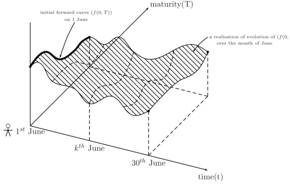
For later empirical implementations it is important to keep in mind how the stochastic dynamic system (4) should be interpreted. Suppose our observation period is 1st June to 30th June, and we have daily observations. On the first of June we have a zero coupon forward curve, f(0, T) (T indicates maturity), reconstructed from a whole set of (noisily)
1The instantaneous spot rate of interest, rt, is treated as unobserved since the shortest rate we observe in
most markets is a 30-day rate. In many empirical studies in finance this latter rate is treated as a proxy forrt. Part of our contribution is the development of a methodology that avoids such an approximation. We should however also point out that [7] discusses situations in which certain market observed short rates (such as 30-day and 90-day rates) are reasonable proxies forrt.
2Recall that
P(t, T) = exp
−tTf(t, u)du
observed forward rates. It is more likely that agents observe the prices of available zero-coupon bonds, however, since there is a one-to-one correspondence between these prices and forward rates, we may as well assume that the agents have access to the latter (forward rates can be reconstructed from observable data). Whether we take available bond prices or forward rates as the observed quantities, these have to be reconstructed from actually accessible data, and so such observations have to be considered as noisy. In spite of the fact that the forward rates are noisy, we take the reconstructedf(0, T) as the ”true” zero coupon yield curve on 1st June. This viewpoint is consistent with the one we shall adopt in setting up the (Bayesian) filtering algorithm (see Remark 2.4).
The SDE system (4) that we are considering tells us how the zero coupon forward curve of 1 June will be projected over the month of June under the proposed forward rate volatility function. Recall that under the assumptions of the model, the evolution of the forward curve on any day is driven by that of the state variables.
This evolution of the initial forward curve can be depicted as shown in Fig. 1.
1
stJune
maturity(T)
time(t)
30
thJune
k
thJune
initial forward curve (f(0, T)) on 1 June
a realisation of evolution of (f(0, T)) over the month of June
Figure 1: The Evolution of the Forward Curve
•
Solid curve — initial (reconstructed from forward rates of many maturities) forward curve
•
Dashed curves — realisations of the evolution of
f
(0
, T
)
In order to focus on perhaps the simplest filtering problem in the framework of the stochastic dynamical system (4), we shall assume (see (16) below) that the available ob-servations are noisy obob-servations of the forward rate with the fixed maturity τ (one may obviously add noisy observations of forward rates with other maturities as well as of any
other economic quantity, whose dynamics can be derived from (4)).
Since ft = f(t, τ) has to be treated here as an underlying quantity as opposed to a derivative quantity, we have to model its observations under the “historical” or “real world” probability measureP. 3 We shall therefore introduce the “market price of interest rate risk” processψt, that corresponds to the translation of the Wiener process when passing from the measureQtoP, and assume that it satisfies, under the measureP, a mean reverting diffusion model. The market price of interest rate risk is essentially the additional compensation that a rational investor, operating under conditions of absence of arbitrage, would require for bearing an additional unit of interest rate risk as measured by a unitary increase in volatilty of the forward rate curve (see e.g. [4]).
Denote then byXtthe “state” process
Xt:= [ft, rt, ψt] (8)
and, given a (large)H >0 and a (small) >0, let
χ(X) = 1 if max{|ft|,|rt|} ≤H 0 if min{|ft|,|rt|} ≥H+; else a Lipschitz interpolation
¯ χ(ψ) = 1 if |ψ| ≤H 0 if |ψ|> H+ H+−|ψ| if H <|ψ|< H+ (9) Under the measure P with Wiener process wt = ˜wt− 0tψsds, we now let the processes
ft, rt, ψt satisfy the dynamics dft= (Dtσ(t, τ;rt, ft) +ψt)σ(t, τ;rt, ft)χ(Xt)dt+σ(t, τ;rt, ft)χ(Xt)dwt drt= [At+Btrt+Ctft+ψtσ(t, t;rt, ft)]χ(Xt)dt+σ(t, t;rt, ft)χ(Xt)dwt dψt=κ ¯ ψ−ψt ¯ χ(ψt)dt+b|ψt|γχ¯(ψt)dwt (10)
where the totality of the parameters is given by the vector
θ:= (a0, a1, a2, δ, κ,ψ, b, γ, λ¯ ) (11)
and each of them is supposed to take values in a compact subset of the positive halfline. With the vectorXt as in (8), we shall write the dynamics in (10) in compact form as
dXt=Ft(Xt)dt+Gt(Xt)dwt (12)
where Ft(·) and Gt(·) are implicitly defined in (10). In what follows, the generic i−th
(i= 1,2,3) components ofFt(·) andGt(·) will be denoted byFt(i)(·) andG(ti)(·) respectively. We have
Proposition 2.1 The system (10) (equivalently (12)) has a unique strong and bounded so-lution.
3On the other hand, if one takes as observations any of the derivative quantities, one would have the choice
(depending on the intended application) of modelling their observations either under the martingale measureQ
Proof : The boundedness of the solution follows from the truncation factors in the coeffi-cients. It then suffices to show that, for a bounded solution, the drift and diffusion coefficients in the three equations in (10) are globally Lipschitz and for this purpose it is easily seen that it suffices to show the Lipschitzianity with respect to the spatial variable.
For the first drift coefficient we have
|[Dtσ(t, τ;r, f) +ψ]σ(t, τ;r, f)χ(X)−[Dtσ(t, τ;r, f) +ψ]σ(t, τ;r, f)χ(X)|
≤C σ2(t, τ;r, f)χ(X)−σ2(t, τ;r, f)χ(X)+|σ(t, τ;r, f)ψχ(X)−σ(t, τ;r, f)ψχ(X)| (13) withCa constant and from here the Lipschitzianity follows by the boundedness ofσ(·), χ(·) andψ and the Lipschitzianity ofσ(·) and χ(·) (recall that r, f andψ are solutions of (10) and therefore bounded).
Coming to the second drift term we have
|[At+Btr+Ctf+ψtσ(t, t;r, f)]χ(X)−[At+Btr+Ctf+ψtσ(t, t;r, f)]χ(X)| ≤ |At| |χ(X)−χ(X)|+|Bt| |rχ(X)−rχ(X)|
+|Ct| |f χ(X)−fχ(X)|+|σ(t, t;r, f)ψtχ(X)−σ(t, t;r, f)ψtχ(X)|
(14) The functionAt is an input and is bounded, uniformly int, together with Btand Ct. The Lipschitzianity then follows for the same reasons as before.
For the last drift term the Lipschitzianity follows again straightforwardly for the same reasons as before since
κ¯
ψ−ψχ¯(ψ)−κψ¯−ψχ¯(ψ)≤C (|χ¯(ψ)−χ¯(ψ)|+|ψχ¯(ψ)−ψχ¯(ψ)|) (15) Finally, the Lipschitzianity of the diffusion coefficients follows by complete analogy with the drift coefficients.
Remark 2.2 In the literature one can find results on the existence of a strong solution to equations of the form (4) with volatilities according to (3) and (5) (see e.g. [10]). These results hold however for specific ranges of the parameterδ in (5). In our applicationδ may take any positive value and so we preferred to introduce the Lipschitz truncation factors (9) to ensure in any case the existence of a strong and bounded solution. From a practical point of view this truncation is hardly any restriction at all.
Model (12), resulting from (10) is a minimal Markovian model for the term structure of interest rates : the dynamics of the various other forward ratesf(t, T) with generic maturity
T ( as well as the corresponding zero-coupon bond prices) can be derived from the first equation in (4) and from (7), whose dynamics depend only on the vectorXt. In what follows we shall denote byX the compact subset of IR3 for whichXt∈ X.
In line with the foregoing, we shall assume that agents have access to noisy observations offt=f(t, τ). Denoting the observation process by yt, we assume that it satisfies
with ˆ >0 small and ˆwta P−Wiener, independent ofwt.
The goal here is a recursive Bayesian-type estimation ofXtandθon the basis of the past and present observations ofyt, i.e. the combined filtering and parameter estimation of (Xt, θ),
givenFty, which is the filtration generated by the processyt. The most complete solution to
this problem is the recursive computation of the conditional joint distributionp(Xt, θ| Fty). This is a highly nonlinear filtering problem and so in section 3 we shall compute a weak approximation top(Xt, θ| Fty) in the sense that we shall compute an approximation of the
conditional expectation
EΓ(¯ Xt;θ)| Fty=
¯
Γ(X;θ)dp(X;θ| Fty) (17) where, for eachθ, ¯Γ(·;θ) is Lipschitz. The approximation is by discretization in time, which is motivated not only by the difficulty of computing (17) exactly, but also by the fact that, in reality, yt is observed in discrete time. Additional possible approximations will also be
mentioned in section 3
Remark 2.3 Since the solution Xt of (12) takes values in the compact set X, we may, without changing the value in (17), assume that Γ(¯ X;θ) = 0 for X ∈ X. Notice also that from the econometric literature one has an indication of what could be possible values of the parameter vector θ. We shall thus assume thatθ takes already from the outset only a finite number of possible values to which we may assign a uniform prior. This implies that the time discretization below concerns only the processXt and, to emphasize this fact, we shall putΓθ(X) := ¯Γ(X;θ)so that, instead of (17), we shall compute/approximate
E{Γθ(Xt)| Fty} (18)
Remark 2.4 Stochastic filtering can be viewed as a dynamic generalization of Bayesian statistics. The “prior distribution” in this dynamic setup is given by the joint distribution of the (unobservable) state processXtand of the parameter vectorθ. This distribution is implied by the dynamic model for Xt (see (10) and (12)) and by the prior distribution onθ. This joint prior distribution is then successively updated on the basis of empirical data, namely of the noisy observations yt of ft. Analogously to classical Bayesian statistics, also in its dynamic generalization the “prior” is specified on the basis of extra-experimental information and/or on the basis of prior empirical information. As explained in the paragraph below equation (6), this is also the sense in which our double use of observations of forward rates is being interpreted : the one time initial observations off(0, t), f(0, τ), fT(0, t)correspond to “prior” empirical information which is used, see (6), to determine the functionAtthat is part of the dynamic model forXt (see (10)), and thus of the “prior” forXt. The successive noisy observationsytof fton the other hand constitute the successively increasing empirical information, on the basis of which the prior of (Xt, θ)is being updated.
We want to point out that, in Bayesian statistics, the current distributions turn out to be more informative, if one is able to assign a more informative prior. To this effect notice that, although the solution of (12) takes values in the compact setX, there is no guarantee on the
positivity of the instantaneous ratesrt andft. Since these rates are essentially positive, we
should get more informative results if the “prior”, i.e. our dynamic model forXtguarantees positivity of these rates. For this purpose notice next that, if two quantities are in a one-to-one correspondence with each other, observing one-to-one of them or updating the distribution of one of them turns out to be equivalent to observing the other or updating its distribution respectively. We may therefore apply to the ratesrtandftan invertible transformation that transforms them into positive rates. For this purpose we use theC2−transformation
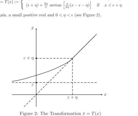
¯ x=T(x) := x if x≥+η (+η) +2πη arctan π 2η(x−−η) if x < +η (19) whereis, again, a small positive real and 0< η < (see Figure 2).
x
¯
x
ε
+
η
ε
ε
+
η
Figure 2: The Transformation ¯
x
=
T
(
x
)
Define ρt := T(rt), φt :=T(ft) and notice that, with the same H as in (9), ρt, φt ≥ T(−H−)> and, on [+η, H], we haveρt=rt, φt=ft. Putting ¯Xt:= [φt, ρt, ψt], we may, with some abuse of notation, also write ¯Xt =T(Xt) and, applying Ito’s rule, obtain
from (12)
dX¯t= ¯Ft(Xt)dt+ ¯Gt(Xt)dwt (20)
where thei−th (i= 1,2,3) components of ¯Ft(·) and ¯Gt(·) are
¯ Ft(i)(Xt) = Ft(i)(Xt) if i= 3 ˙ T(Xt(i))Ft(i)(Xt) +12T¨(Xt(i))(G(ti))2(Xt) if i= 1,2 ¯ G(ti)(Xt) = G(ti)(Xt) if i= 3 ˙ T(Xt(i))Gt(i)(Xt) if i= 1,2 (21)
and they are bounded since all the individual factors on the right in (21) are. SinceT(·) is invertible, the Ito process ¯Xtin (20) can be represented as solution of
Proposition 2.5 Equation (22) admits a unique strong solution.
Proof : Notice first from (19) that the inverse transformationT−1(¯x) is given by
T−1(¯x) = ¯ x x¯≥+η (+η) +2πηtan π 2η(¯x−−η) <x < ¯ +η
and is Lipschitz so that Ft(i)T−1( ¯X) and G(ti)T−1( ¯X) are also Lipschitz in addition to being bounded. To obtain the global Lipschitzianity of the coefficients in (22) and thus the existence of a strong solution, by (21) it suffices thus to show Lipschitzianity and boundedness of ˙TT−1(¯x) and ¨TT−1(¯x). This follows immediately from their explicit expression, namely ˙ TT−1(¯x)= 1 x¯≥+η 1 1+[tan(π 2η(¯x−−η))]2 <x < ¯ +η ¨ TT−1(¯x)= 0 x¯≥+η π ηtan[2πη(¯x−−η)] 1+[tan(π 2η(¯x−−η))]2 2 <x < ¯ +η
In what follows we shall always refer to the same model (12) also in the case when we apply the transformationT(·). In this latter caseXtstands for ¯Xt, and the functionsFt(X)
andGt(X) then correspond to ¯FtT−1( ¯X)and ¯GtT−1( ¯X)respectively. Similarly, ft in equation (16) stands forφtin case we apply the transformationT(·).
Notice that alternative approaches to obtain positive rates can be found in the recent literature (see e.g. [13]).
Notice finally that the filtering approach to HJM term structure models can also be seen as a possible way to overcome consistency problems in the calibration of HJM models (for the latter see e.g. the overview in [5]).
3
Time discretization and convergence results
In the following we implicitly assume that a generic value of θ has been fixed. Consider the partition of [0, T] into subintervals of the same width ∆ = NT and perform an Euler discretization of (12), namely
XnN+1−XnN =FnXnN∆ +GnXnN∆wn (23) with ∆wn =w(n+1)∆−wn∆. Notice that, while the solution of the continuous-time model (12) is bounded, its discretized version (23) does not guarantee boudedness of (XnN). Denote byXN
t the piecewise constant time interpolation ofXnN, namely
XtN := XN n n∆≤t <(n+ 1) ∆ XN N t=T (24)
Consider next a Girsanov-type change of measure which allows us to transform the orig-inal filtering problem into one with independent state and observations. Denote byP0 the measure under which yt is a Wiener process, independent of Xt and thus also of XtN. In
fact, the change of measure affects only the distribution of yt and not also of Xt . The
corresponding Radon-Nikodym derivative is
dP dP0 = exp 1 ˆ 2 T 0 fsdys− 1 2ˆ2 T 0 f 2 sds (25)
Analogously, denote byPN the measure under which y
tsatisfies the equation
dyt=ftNdt+ ˆdwtN (26)
withwN
t a PN−Wiener process and where, with some abuse of notation, we denote byftN
the first component ofXN
t , truncated upon exit from [−(H+),(H+)] (H andare the
same as in (9)); as a consequence, in what follows fN
t will be treated as having the same
bounds as ft. We thus have that, underPN, yt has the same form as under P, but as a
function of the discretized state.
Applying the so-called Kallianpur-Striebel formula (see [16]), the filter in (18) can be expressed as E{Γθ(Xt)| Fty}= E 0Γ θ(Xt)dPdP0|Fty E0dPdP0|Fty (27)
It follows that it suffices to approximate, for each value of θ,
Vt(Γθ;y) :=E0 Γθ(Xt) dP dP0|F y t (28) (the denominator in (27) is in fact simplyVt(1;y)).
Define zt:=E0 dP dP0|Ft = exp t 0 1 ˆ 2fsdys− 1 2ˆ2 t 0 fs2ds (29) zNt :=E0 dPN dP0|Ft = exp t 0 1 ˆ 2f N s dys− 1 2ˆ2 t 0 (f N s )2ds (30) whereFt=Fty∨ FX
t . By analogy to (28) define, forN ∈IN, VtN(Γθ;y) :=E0
Γθ
XtNzTN|Fty (31) By the ”smoothing property” of conditional expectations we have
Vt(Γθ;y) =E0{Γθ(Xt)zt|Fty}, VtN(Γθ;y) =E0ΓθXtNzNt |Fty (32) We first have the following
Proposition 3.1 The processes{Xt} and XtNsatisfy, fort∈[0, T] EXt−XtN 4≤ K∆2 and E0Xt−XtN 4≤ K∆2
Proof : The proof can easily be adapted from [12], where the components of XN t are
not truncated, while here we have truncated the first component fN
t . Notice however
that, given the recursions (23) and our assumptions, the difference in fourth mean of the truncated and non-truncated values of fN
t is, for all t ∈ [0, T], bounded from above by E
Fn(1)(·)∆ +G(1)n (·)∆wn 4
≤const·F(1)4+G(1)4∆2 and the coefficient of ∆2 in this latter quantity is bounded due to the fact thatF and Gare bounded by definition and this also in the case when we apply the transformation T(·) in (19) (see (21) and the proof of Proposition 2.5).
Notice that, according to Remark 2.3, the value ofVN
n∆(Γθ;y) in (31) does not change if
we change the values ofXN
t outside ofX. Consequently, we shall truncate the processXtN as
soon as it exits fromXand denote byXnthe so truncated process (Xn(i)will denote thei−th
(i= 1,2,3) component ofXn and notice that forfnN =fn=Xn(2) we have already used this
truncation after (26)). The processXnis now bounded Markov with a well-defined transition kernelP(Xn+1|Xn). The explicit expression ofP(Xn+1|Xn) is somewhat complicated but,
for the actual calculations, we need its expression only in the interior of X and there it is given by P(Xn+1|Xn) = 1 2π(G(1)n )2(Xn)∆ exp − Xn(1)+1−Xn(1)−Fn(1)(Xn)∆ 2 2(G(1)n )2(Xn)∆ · 3 i=2 δ Xn(i+1) −Xn(i)−Fn(i)(Xn)∆ −G(i) n (Xn))· Xn(1)+1−Xn(1)−Fn(1)(Xn)∆ G(1)n (Xn) · 3 i=1 1[−(H+),(H+)] Xn(i+1) (33)
We also make the following assumption, which is in line with our observation model (16)
Assumption A.1 : The actually observed trajectory (yt) satisfies, forn= 0,· · ·, N−1, sup
s,t∈[n∆,(n+1)∆]
|ys−yt| ≤K∆1/2
Lemma 3.2 Given an observed trajectoryys(s≤t)satisfying A.1, we have fort=n∆ E0zt2|Fty≤K(y) ; E0(zNt )2|Fty≤K(y) (34)
E0zt−ztN|Fty≤K¯(y)·∆12 (35)
whereK(y),K¯(y)depend only on the observed trajectoryys,s≤t.
Proof. We start with the proof of the first inequality in (34). Using the stochastic integration by parts formula and the fact thatXn= [fn, rn, ψn] is bounded together with the coefficients
Ft(i)(·), Gt(i)(·) (i= 1,2,3), we have E0zt2| Fty=E0 exp 2 ˆ 2 t 0 fsdys− 1 ˆ 2 t 0 f 2 sds | Fy t ≤E0 exp 2 ˆ 2ftyt− 2 ˆ 2 t 0 ysdfs | Fy t ≤K(y)E0 exp −2 ˆ 2 t 0 ysF (1) s (Xs)ds− 2 ˆ 2 t 0 ysG (1) s (Xs)dws | Fy t ≤K¯(y)E0 exp t 0 Hs(y)dws− 1 2 t 0 H 2 s(y)ds exp 1 2 t 0 H 2 s(y)ds ≤K˜(y) (36)
for appropriate constants K(y),K¯(y),K˜(y) and an adapted bounded process Hs(y) that
depends on the observed trajectory ofy (recall that, underP0, the processesXtandytare
independent).
Coming to the second inequality in (34) and recalling that the values offnN are bounded, we have, fort=n∆ and with ∆yi+1:=y(i+1)∆−yi∆,
E0(ztN)2| Fty = E0 exp 2 ˆ 2 n−1 i=0 fiN∆yi+1− 1 ˆ 2 n−1 i=0 (fiN)2∆ | Fy t ≤ E0 exp 2 ˆ 2 n−1 i=0 fiN∆yi+1 | Fy t ≤K(y) (37)
Next we come to (35). Using |ex−ey| ≤ |x−y| |ex+ey| and (34) we obtain E0|zt−ztN| | Fty ≤ K(y) E0 | t 0 fs−fsN dys|2 + 14| t 0 fs2−(fsN)2ds|2 | Fy t 1/2 (38)
By Proposition 3.1 , the fact that without loss of generality we may assume ∆<1, and the independence, underP0, of the processesXtand yt, it suffices to show that
E0 | t 0 fs−fsN dys|2| Fty ≤K¯(y) ∆ (39) For this purpose, putting ∆yi+1=y(i+1)∆−yi∆, we use the stochastic integration by parts
formula as well as the fact that
fnyn∆= n−1 i=0 fi+1∆yi+1+ n−1 i=0 yi∆fi+1 (40)
together withy0= 0 to obtain, fort=n∆, (n=t/∆), | n∆ 0 fs−fsN dys|2=|yn∆fn∆− n∆ 0 ysdfs− n−1 i=0 fi∆yi+1|2 =|yn∆fn∆− n∆ 0 ysdfs− n−1 i=0 fi+1∆yi+1+ n−1 i=0 ∆fi+1∆yi+1|2 ≤K|yn∆(fn∆−fn)|2+K| n−1 i=0 yi+1∆fi+1− (i+1)∆ i∆ ysdfs ! |2 ≤K1(y) (fn∆−fn)2+K1| n−1 i=0 yi+1∆fi+1− (i+1)∆ i∆ yi+1dfs ! |2 +K2| n−1 i=0 (i+1)∆ i∆ (yi+1−ys)dfs|2=I+II+III (41)
To obtain (39) it suffices now to show that a similar relation holds when replacing the
|t 0 fs−fN s
dys|2 there by the expressions corresponding toI, II,andIII respectively. By Proposition 3.1 the expression corresponding toI is immediately seen to be bounded by ¯K1(y)∆ for a suitableK1(y).
For the expression corresponding toII we have
E0 | t/∆−1 i=0 yi+1∆fi+1− (i+1)∆ i∆ yi+1dfs ! |2| Fy t =E0 t/∆−1 i=0 yi+1 Fi(1)(Xi)∆ +G(1)i (Xi)∆wi − (i+1)∆ i∆ Fs(1)(Xs)ds− (i+1)∆ i∆ G(1)s (Xs)dws | Fy t 2 ≤2E0 t/∆−1 i=0 yi+1 (i+1)∆ i∆ Fi(1)(Xi)−Fs(1)(Xs) ds ! | Fy t 2 +2E0 t/∆−1 i=0 yi+1 (i+1)∆ i∆ G(1)i (Xi)−G(1)s (Xs) dws ! | Fy t 2 ≤2 maxi,j|yi·yj|E0 t/∆−1 i=0 (i+1)∆ i∆ LF(∆ +Xi−Xs)ds !2 + t/∆−1 i,j=0 (i+1)∆ i∆ LF(∆ +Xi−Xs)ds ! · (j+1)∆ j∆ LF(∆ +Xj−Xs)ds ! + t/∆−1 i=0 (i+1)∆ i∆ L 2 G(∆ +Xi−Xs)2ds ! (42) where we have used the fact that, under P0, the processes Xt and yt are independent so
that conditioning on Fty is equivalent to fixing a trajectory of y. Furthermore, we have used the global (also with respect to the time variable) Lipschitzianity ofFt(1)(·) andG(1)t (·) (Lipschitz constants LF and LG respectively) and for the rightmost part we computed the
expectation of the conditional expectation exploiting the property that E0 (i+1)∆ i∆ G(1)i (Xi)−G(1)s (Xs) dws| Fi∆ = 0 and that E0 (i+1)∆ i∆ G(1)i (Xi)−G(1)s (Xs) dws !2 = (i+1)∆ i∆ E0 G(1)i (Xi)−G(1)s (Xs) 2 ds
Notice next that, fors∈[i∆,(i+ 1)∆) we haveXN
s =Xi so thatXi−Xs=XsN−Xs
and therefore, by Proposition 3.1 , E0{Xi−Xs} ≤ K√∆, E0Xi−Xs2 ≤ K∆. Assuming without loss of generality that ∆< 1, we can then continue the above relation (42) to become expression II ≤K(y)L2F∆2+ 2∆5/2+ ∆3+L2 F ∆2+ 2∆5/2+ ∆3 +L2G∆ + 2∆3/2+ ∆2≤K¯(y)·∆ (43)
for suitableK(y),K¯(y) depending on the observed trajectory ofy. Finally, for the expression corresponding toIII we have
E0 | n−1 i=0 (i+1)∆ i∆ (yi+1−ys)dfs|2| Fty =E0 | n−1 i=0 (i+1)∆ i∆ (yi+1−ys) Fs(1)(Xs)ds−Gs(1)(Xs)dws |2| Fty ≤2E0 n−1 i=0 (i+1)∆ i∆ |yi+1−ys| |Fs(1)(Xs)| ds !2 | Fy t +2E0 n−1 i=0 (i+1)∆ i∆ (yi+1−ys)G(1)s (Xs)dws !2 | Fy t ≤K˜∆T||F(1)||2+T||G(1)||2≤K¯ ·∆ (44)
where we have used assumption A.1 and the boundedness of F(1)(·) and G(1)(·) (norms
||F(1)||and||G(1)||).
Theorem 3.3 For each n= 0,1, ..., N, for t =n∆, for each observed trajectoryys, s≤t satisfying A.1 and for each value of θ
Vt(Γθ;y)−VN
t (Γθ;y)≤K1(y)∆12. (45)
whereK1(y)depends only on the observed trajectory ys,s≤t. Proof. We have Vt(Γθ;y)−VtN(Γθ;y)≤E0Γθ(Xt)zt−Γθ(XtN)ztN|Fty ≤E0ztΓθ(Xt)−Γθ(XN t )|Fty +E0Γθ(XN t )zt−ztN|Fty (46)
Applying H¨older’s inequality and the fact that Γθ(·) is, uniformly inθ(recall thatθ takes a
finite number of values) Lipschitz (withL−constant ˆΓ) and bounded (by ˜Γ), (46) is majorized by E0zt2|Fty12ΓˆE0X t−XtN 212 + ˜ΓE0zt−ztN|Fty. (47) By Lemma 3.2 and Proposition 3.1 we then obtain the thesis.
Remark 3.4 Theorem 3.3 implies convergence of the filter for each observed trajectory. This is a stronger form of convergence than those in the traditional filtering literature (see e.g.[19]), where convergence is obtained in the mean with respect to y.
Consider next the sequence of nonnegative measures qn(B;yn), where B denotes the
generic Borel subset ofX and yn = (y∆
1,· · ·, yn∆) with yn∆ :=yn∆−y(n−1)∆, and that are
recursively defined by q0(B) :=p0(B) qn+1 B;yn+1:= B Xexp 1 ˆ 2fny ∆ n+1− 1 2ˆ2f 2 n∆ P(Xn+1|Xn)dqn(Xn;yn)dXn+1 (48) wherep0is the initial distribution andfn corresponds toXn(1), which is also the same asftN
in (26) and (30).
Proposition 3.5 For any bounded functionΨwe have E0Ψ (Xn)zTN|Fny∆=
XΨ (X)dqn(X;y
n). (49)
For a proof see e.g. [1].
Applying this proposition we immediately obtain (writingVnN for theVnN∆(31))
VnN(Γθ;y) =
XΓθ(X)dqn(X;y
n) (50)
for n = 0,1, ..., N and this also implies that, when computing VN
n (Γθ;y), we do not lose
information by considering onlyyn instead of the entire filtrationFny∆.
Using (50) and (27) it is easily seen that the measures qn(B;yn) can be given the
inter-pretation of unnormalized conditional distributions. To determine the time discretized filter it suffices thus to compute the recursions (48). This is still an infinite-dimensional problem and so further approximations are needed, specifically discretizations in the spatial variable (quantization). This can be done in a variety of ways, for which we refer e.g. to [1],[12], [17], [18], [20],[22], [23]. In particular, for problems that are already reduced to discrete time, in [20],[22], [23] a specific methodology is described to arrive at a finite-dimensional approximating filter. Alternatively, always for problems already in discrete time, one could also use the recent so-called “particle approach” to nonlinear filtering, that is based on a simulation methodology (see e.g.[11]).
4
Conclusion
We have considered a version of the Heath-Jarrow-Morton model with a volatility depending on time-to-maturity, the instantaneous spot rate and one fixed maturity forward rate. We have seen how estimation of this model may be set up as a non-linear filtering problem under the historical measure. We have proposed a framework in which a recursive (Bayesian-type) filtering algorithm may be developed.
We have provided convergence results that demonstrate the consistency of the discretized filtering model with the original continuous time counterpart.
Future research needs to focus on actual implementation of the filtering framework pro-posed here. Results of [3] using a recursive (Bayesian) filtering algorithm for estimation in a model of the instantaneous spot rate of interest indicate the feasibility of this general approach.
References
[1] A.Bensoussan, W.Runggaldier, An approximation method for stochastic control prob-lems with partial observation of the state - a method for constructing−optimal controls, Acta Appl. Math., 10 (1987), 145-170.
[2] R.Bhar, C.Chiarella, N.El-Hassan, X.Zheng,The Reduction of Forward Rate Dependent Volatility HJM Models to Markovian Form: Pricing European Bond Options, Journal of Computational Finance, 3(3), 47-72, 2000.
[3] R. Bhar, C. Chiarella, W. Runggaldier,Estimation in Models of the Instantaneous Short Term Interest Rate by use of a Dynamic Bayesian Algorithm, QFRG Working Paper, University of Technology, Sydney, 2001.
[4] T.Bj¨ork, Arbitrage Theory in Continuous Time, Oxford University Press, 1998. [5] T.Bj¨ork, A geometric view of interest rate theory, SSE/EFI Working Paper Series in
Economics and Finance No 419, Dec. 2000. To appear in Handbook of Mathematical Finance, Cambridge University Press.
[6] T.Bj¨ork, L.Svensson, On the existence of finite dimensional realizations for nonlinear forward rate models, Mathematical Finance, 11 (2), 205-243, 2001.
[7] D.A.Chapman, J.B.Long Jr., N.D.Pearson, Using Proxies for the Short Rate : When Are Three Months Like an Instant ?, Review of Financial Studies, 12, 763-806, 1999. [8] C.Chiarella, O.K.Kwon, Forward rate dependent Markovian transformations of the
Heath-Jarrow-Morton term structure model, Finance and Stochastics, 5, 237-257, 2001. [9] C.Chiarella, O.K.Kwon, Classes of Interest Rate Models under the HJM Framework,
Asia Pacific Financial Markets, 8, 1-22, 2001.
[10] G.Deelstra, F.Delbaen,Convergence of Discretized Stochastic (Interest Rate) Processes with Stochastic Drift Term, Appl. Stoch. Models Data Anal. 14, 77-84, 1998.
[11] P.Del Moral,Measure valued processes and interacting particle systems. Applications to nonlinear filtering problems, Ann.Appl.Probab., 8, 438-495, 1998.
[12] G.B. Di Masi, M.Pratelli, W.J.Runggaldier, An Approximation for the Nonlinear Fil-tering Problem, with Error Bound, Stochastics, 14, 247-271, 1985.
[13] B.Flesaker, L.P. Hughston,Positive interest, Risk 9, 46-49, 1996.
[14] D.Heath, R.Jarrow, A.Morton,Bond Pricing and the Term Structure of Interest Rates: A New Methodology for Contingent Claim Valuation, Econometrica, 60(1),77-105, 1992. [15] T.S.Y.Ho, S.B.Lee,Term Structure Movements and Pricing Interest Rate Contingent
Claims,Journal of Finance, 1011-1029, 1986 .
[16] G.Kallianpur, C.Striebel,Estimation of stochastic processes. Arbitrary system processes with additive white noise observation error, Ann. Math. Stat., 39 (1968), 785-801. [17] H. Korezlioglu, W.J. Runggaldier,Filtering for Nonlinear Systems Driven by Nonwhite
Noises : an Approximation Scheme, Stochastics and Stochastics Reports, 44 (1993), 65-102.
[18] H.J.Kushner, P.Dupuis,Numerical Methods for Stochastic Control Problems in Contin-uous Time, Springer-Verlag, New York 1992.
[19] R.S. Liptser, O. Zeitouni, Robust Diffusion Approximation for Nonlinear Filtering, J.Math.Systems, Estimation and Control, 8 (1998), 1-22.
[20] S. Pasquali, W.J. Runggaldier,Approximations of a controlled diffusion model for renew-able resource exploitation, Kluwer Volume on Markov Processes and Controlled Markov Chains, in print.
[21] P.Ritchken, L.Sankarasubramanian, Volatility structures of forward rates and the dy-namics of the term structure, Mathematical Finance, 5 (1), 55-72, 1995.
[22] W.J. Runggaldier, On the construction of −optimal strategies in partially observed MDP’s, Annals of Oper. Res., 28, 81-96, 1991.
[23] W.J. Runggaldier, O. Zane,Approximations for Discrete-Time Adaptive Control : Con-struction of −Optimal Controls, Math. Control Signals Systems, 4, 269-291, 1991. [24] O.Vasicek,An Equilibrium Characterisation of the Term Structure, Journal of Financial