Mining gold: Improving simulation-based inference
with latent information
Johann Brehmer, Kyle Cranmer, Siddharth Mishra-Sharma New York University
[email protected] Felix Kling SLAC Gilles Louppe University of Liège
Abstract
We summarize and discuss new inference techniques for systems that are described by a simulator with an intractable likelihood function. The key idea is that addi-tional information that characterizes the latent process can often be extracted from the simulator. It can then be used to augment the training data for neural surrog-ates of the likelihood function. These methods have been applied to problems in particle physics and astrophysics, and the initial results demonstrate their potential to improve sample efficiency and quality of inference.
1
Simulation-based inference
Phenomena across many domains of science are most accurately described by complicated computer simulations. These simulators typically implement aforward mode: given some model parametersθ
as input, they generate potential outcomes or observationsx, sampled from a probability density or likelihood functionx∼p(x|θ). Often the true values of these model parametersθare not known, and the inverse problem of inferring the likely values ofθfrom measured values of the observablesx
is an important goal. Both in a frequentist and a Bayesian setup, the central object for this inference task is the likelihood function, which can be schematically written as
p(x|θ) = Z
dz p(x, z|θ). (1)
Here we are integrating over all possible values of the latent variableszthat describe the generative process, andp(x, z|θ)is the joint probability density orjoint likelihood functionof observables and latent variables.
Realistic scientific simulators often involve a large number of latent variables, and the integral over such a high-dimensional space cannot be calculated explicitly (nor can it be sampled efficiently for a fixedx). The likelihood function is therefore intractable. This is a major challenge for scientific inference in fields ranging from particle physics to cosmology, epidemiology, genetics, and climate science.
Inference in this case requiressimulation-based (orlikelihood-free) inference techniques. Some approaches, including the well-known Approximate Bayesian Computation (ABC) technique [1, 2] as well as methods based on density estimation [3], rely on reducing the observations to low-dimensional summary statistics. Standard choices of these summary statistics discard information and reduce the power of a measurement. In another approach, neural networks are trained as surrogates for the likelihood, the likelihood ratio, or the posterior [4–30]. Usually these methods are agnostic about the latent process in the simulator and only use its outputxduring training.
Here we review a recently proposed family of techniques that extracts more information from the simulator and uses this augmented data to train neural networks to either learn the likelihood or likelihood ratio function efficiently or to define powerful summary statistics that are statistically optimal in a well-defined approximation [31–34]. In Sec. 3 we point to software tools that automate this process. We then discuss the application of these ideas to various problems in Sec. 4. We conclude with a brief discussion of this approach in Sec. 5.
This submission reviews the ideas originally presented in Refs. [31–34] and presents an overview of the application of these ideas to the physical sciences [35–37]. It is intentionally kept brief, aiming for an “extended abstract” style. For a camera-ready version, we would expand it into a more typical paper form and add new, so far unpublished results demonstrating the power of these methods.
2
Algorithms
Extracting additional information from simulations. When running a simulator for model para-metersθ, it is often possible to extract and save two additional quantities, thejoint likelihood ratio
r(x, z|θ)and thejoint scoret(x, z|θ)defined as [31–33]
r(x, z|θ) = p(x, z|θ)
pref(x, z)
and t(x, z|θ) =∇θlogp(x, z|θ). (2) Both quantities depend on the latent variables that characterize a particular run of the simulator. The joint likelihood ratio quantifies how likely a particular simulation run (including all latent variables) is compared to a reference distributionpref(x, z), while the joint score quantifies how much more or less likely it becomes under infinitesimal changes of the model parameters.
Efficiently learning the likelihood (ratio). The joint likelihood ratio and the joint score can then be used to construct certain loss functionalsL[g(x, θ)], where the test functiong(x, θ)is only a function of the observablesxand parametersθ(not of the latent variablesz). It can be shown that these loss functionals are minimized by the likelihood functionarg mingL[g(x, θ)] = p(x|θ)or the likelihood ratio functionarg mingL[g(x, θ)] =r(x|θ)≡p(x|θ)/pref(x), depending on the loss function [31–34]. This minimization is implemented through machine learning: a neural network implements the variational familyg(x, θ), and the loss functional is numerically minimized through stochastic gradient descent. In this way the neural network learns an approximate version of the likelihood or likelihood ratio function, which are otherwise intractable! We demonstrate this trick in the top left panel of Fig. 1. After an upfront training phase it can be evaluated efficiently and provides the central ingredient to both frequentist [31–33] and Bayesian [30, 37] inference.
Learning locally optimal summary statistics. Alternatively, we can use the joint score to con-struct a loss functional L[g(x)] that is minimized by the score [31–33], arg mingL[g(x)] =
t(x|θref) ≡ ∇θlogp(x|θ)|θref. In a parameter region close to the reference parameter point θref, the components of this vector are the sufficient statistics: reducing a high-dimensional measurement to this low-dimensional vector does not lose any information on the parameters of interest. A neural network trained by minimizing this loss therefore defines an optimal set of summary statistics for frequentist inference based on histograms or ABC [38].
The authors of Ref. [31] have used the metaphor of “mining gold” to describe the extraction of the joint likelihood ratio and joint score from the simulator: while it may require some effort to calculate, it can be very valuable for inference.
3
Automation and tools
General strategies. These inference techniques rely on the ability to calculate the joint likelihood ratio and joint score. This can generally be done in one of three ways [31]:
1. In some simulators, domain knowledge allows us to calculate these quantities manually, either by modifying the simulator code or by extracting the required information from existing simulator output. Often only some steps of the latent process depend on the parameters of interest, which can simplify this calculation substantially.
2. The calculation can be added to an existing simulator via a protocol such as PPX [39]. 3. New simulators can be written within a probabilistic programming frameworks. In this case
the joint likelihood ratio and joint score can be calculated automatically.
MADMINER. The MADMINERlibrary [35] automates all steps of the discussed inference tech-nique for particle physics processes that occur in the ATLAS and CMS experiments in the Large Hadron Collider. The calculation of the joint likelihood ratio and joint score is based on the spe-cific structure of these processes. The library wraps around the particle physics simulators MAD -GRAPH5_AMC [40] and PYTHIA8 [41], supporting almost any relevant high-energy physics scatter-ing process and theories of new physics. It also supports the phenomenological detector simulation DELPHES3 [42], though it is extendable to a full GEANT4-based detector simulation [43] as used by the ATLAS and CMS collaboration. MADMINERis under continuous development and has a growing user base.
Automation for PYRO simulators. As a proof of principle for the automatic computation of the joint likelihood ratio and joint score for general simulators, Ref. [44] provides a framework that calculates these quantities automatically for any simulator in which all stochastic steps are implemented with the PYROlibrary [45].
4
Application to the physical sciences
Toy problems. Reference [31] demonstrated these techniques in two toy problems, including the generalized Galton board and the Lotka-Volterra system of predator-prey dynamics [31]. It was found that using the joint likelihood ratio and joint score during training improves the sample efficiency.
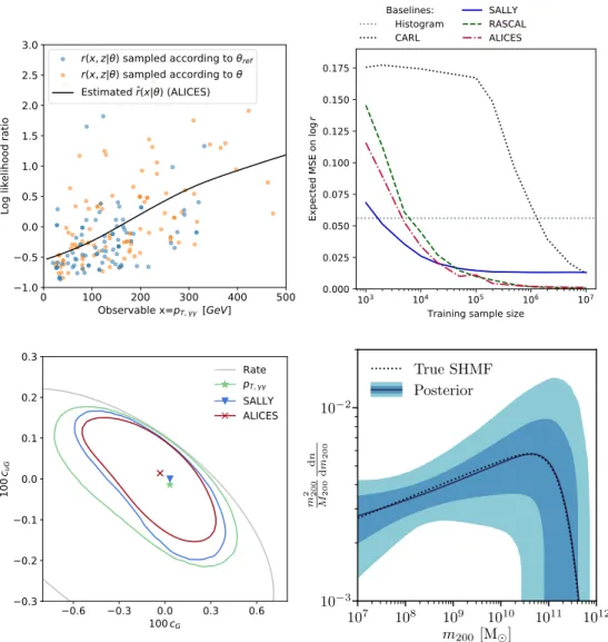
Particle physics. The new techniques have been applied to a number of measurement problems in proton-proton collisions at the Large Hadron Collider, focusing on one of the most interesting problems in particle physics in the coming years: the precision measurement of Higgs boson prop-erties and the search for subtle, “indirect” effects of new physics. The analyzed processes include Higgs production in the “weak boson fusion” mode with a decay into four leptons [32–34], the production of Higgs bosons together withW bosons [36], and Higgs production together with top quarks [35]. In all cases, the new methods were found to substantially improve the sensitivity to the parameters of interest compared to industry standard methods based on summary statistics, as we show top right and bottom left panels of Fig. 1. Ongoing projects use these methods to analyze
CP violation inttH production [46] as well as look for suppressed interference effects inW γ
production. After these phenomenological studies, members of the ATLAS collaboration are now in the process of implementing these techniques into an actual measurement based on real data. On the conceptual side, Ref. [47] compares the new inference techniques to the Matrix Element Method and the Optimal Observable technique, two domain-specific inference methods that also use information that characterizes the latent process.
Cosmology and astrophysics. The nature of dark matter is one of the most intriguing open ques-tions of high-energy physics. Strong gravitational lensing — light patterns emitted from a background galaxy and bent by the gravitational field of another galaxy — will soon offer us a rare chance to search for the effects of the dark matter substructure, i. e. its distribution on small length scales, but teasing out this subtle effect is difficult. In Ref. [37] it was shown how the inference techniques discussed above make such an analysis possible. With this approach, the expected observations from upcoming surveys can be efficiently analyzed, promising the extraction of a maximal amount of information on population parameters describing dark matter substructure, as we demonstrate in the bottom right panel of Fig. 1.
Other fields. We are currently investigating problems from other fields for which these methods may be useful. One particularly interesting system is the simulation of epidemiological systems. Systems biology and climate science might also offer interesting applications.
0 100 200 300 400 500 Observable x=pT, [GeV] 1.0 0.5 0.0 0.5 1.0 1.5 2.0 2.5 3.0
Log likelihood ratio
r(x, z| ) sampled according to ref
r(x, z| ) sampled according to
Estimated r(x| ) (ALICES)
103 104 105 106 107 Training sample size
0.000 0.025 0.050 0.075 0.100 0.125 0.150 0.175 Ex pe cte d MS E on lo gr Baselines: Histogram CARL SALLY RASCAL ALICES 0.6 0.3 0.0 0.3 0.6 100cG 0.3 0.2 0.1 0.0 0.1 0.2 0.3 10 0cuG Rate pT, SALLY ALICES 107 108 109 1010 1011 1012 m200 [M] 10−3 10−2 m 2 200 M 200 d n d m 200 True SHMF Posterior
Figure 1:Top left: Illustration of the new inference techniques in a particle physics problem, the measurement of new physics effects in the production of a Higgs boson with two top quarks. The likelihood ratio as the function of a one-dimensional observable (on thexaxis) is estimated. The dots show the joint likelihood ratio extracted from different runs of the simulator (the training data). The solid line shows the likelihood ratio estimated from the neural network. Figures taken from Ref. [35]. Top right: Performance in a particle physics problem, the measurement of new physics effects in the production of a Higgs boson in the “weak boson fusion” mode with a decay into four leptons. We consider a simplified scenario in which the true likelihood function is tractable. For different methods of likelihood ratio estimation, we show the error of the resulting estimate as a function of training sample size. The new algorithms (red, blue, green) substantially improve the sample efficiency compared to two baselines (grey and black dotted). Based on results in Refs. [32–34]. Bottom left: Performance in a particle physics problem, the measurement of new physics effects in the production of a Higgs boson with two top quarks. We show expected confidence limits in terms of two model parameters (xandyaxis) based on a traditional histogram-based method (green), the optimal summary statistic defined through the new techniques presented here (blue), and likelihood ratio estimation with the new techniques (red). The new machine learning–based techniques lead to tighter exclusion limits, demonstrating an improvement in inference quality. Figures taken from Ref. [35].Bottom right: Bayesian inference in an astrophysical problem, the measurement of dark matter substructure parameters based on observations of strong gravitational lensing. We show the expected posterior on the dark matter subhalo mass function (solid black) together with 68% and 95% credible intervals. The method faithfully recovers the true function used to generate the data (dotted black). Figure taken from Ref. [37].
5
Discussion
“Mining gold” — extracting additional quantities from a simulator that characterize the latent process, and using this information to train neural networks to learn the likelihood function — has the potential to improve scientific inference for many problems. Unlike traditional likelihood-free inference techniques, in particular ABC, it does not require to compress the data to ad-hoc summary statistics, avoiding the corresponding loss of information. After an upfront training phase, the evaluation of new observations is very efficient, amortizing the cost of inference. Compared to other techniques in which neural networks are trained to learn the likelihood or posterior, the extra information can improve the sample efficiency and thus improve the fidelity of the inference and / or reduce the computational cost. Since this approach focuses on the loss functionals and is agnostic about the model architecture, it is orthogonal to recent improvements in neural density estimators such as normalizing flows, and can easily be applied to these models.
Acknowledgements
We want to thank our co-authors Sally Dawson, Irina Espejo, Joeri Hermans, Samuel Homiller, Juan Pavez, Tilman Plehn, and Markus Stoye. Our work benefitted from many great discussions; while we lack the space to list everyone, we are particularly grateful to Lukas Heinrich, Jan-Matthis Lückmann, and George Papamakarios. We are supported by the National Science Foundation under the awards ACI-1450310, OAC-1836650, and OAC-1841471; through the NYU IT High Performance Computing resources, services, and staff expertise; by the Moore-Sloan data science environment at NYU. KC is also supported through the NSF grant PHY-1505463, FK by NSF grant PHY-1620638.
References
[1] D. B. Rubin: ‘Bayesianly Justifiable and Relevant Frequency Calculations for the Applied Statistician’. The Annals of Statistics 12 (4), p. 1151, 1984. URLhttps://doi.org/10. 1214/aos/1176346785.
[2] M. A. Beaumont, W. Zhang, and D. J. Balding: ‘Approximate Bayesian computation in popula-tion genetics’. Genetics 162 (4), p. 2025, 2002.
[3] P. J. Diggle and R. J. Gratton: ‘Monte Carlo Methods of Inference for Implicit Statistical Models’, 1984.
[4] Y. Fan, D. J. Nott, and S. A. Sisson: ‘Approximate Bayesian computation via regression density estimation’. Stat 2 (1), p. 34, 2013. arXiv:1212.1479.
[5] L. Dinh, D. Krueger, and Y. Bengio: ‘NICE: Non-linear Independent Components Estimation’ , 2014. arXiv:1410.8516.
[6] M. Germain, K. Gregor, I. Murray, and H. Larochelle: ‘MADE: Masked autoencoder for distribution estimation’. 32nd International Conference on Machine Learning, ICML 2015 2, p. 881, 2015. arXiv:1502.03509.
[7] D. J. Rezende and S. Mohamed: ‘Variational inference with normalizing flows’. 32nd Interna-tional Conference on Machine Learning, ICML 2015 2, p. 1530, 2015. arXiv:1505.05770. [8] K. Cranmer, J. Pavez, and G. Louppe: ‘Approximating Likelihood Ratios with Calibrated
Discriminative Classifiers’ , 2015. arXiv:1506.02169.
[9] L. Dinh, J. Sohl-Dickstein, and S. Bengio: ‘Density estimation using Real NVP’ , 2016. arXiv:1605.08803.
[10] B. Paige and F. Wood: ‘Inference networks for sequential monte carlo in graphical mod-els’. 33rd International Conference on Machine Learning, ICML 2016 6, p. 4434, 2016. arXiv:1602.06701.
[11] G. Papamakarios and I. Murray: ‘Fast e-free inference of simulation models with Bayesian conditional density estimation’. In ‘Advances in Neural Information Processing Systems’, p. 1036–1044, 2016.
[12] O. Thomas, R. Dutta, J. Corander, S. Kaski, and M. U. Gutmann: ‘Likelihood-free inference by ratio estimation’ , 2016. arXiv:1611.10242.
[13] B. Uria, M.-A. Côté, K. Gregor, I. Murray, and H. Larochelle: ‘Neural Autoregressive Distribu-tion EstimaDistribu-tion’ , 2016. arXiv:1605.02226.
[14] A. Van Den Oord, N. Kalchbrenner, O. Vinyals, L. Espeholt, A. Graves, and K. Kavukcuoglu: ‘Conditional image generation with PixelCNN decoders’. Advances in Neural Information
Processing Systems p. 4797–4805, 2016. arXiv:1606.05328.
[15] A. van den Oord, S. Dieleman, H. Zen, et al.: ‘WaveNet: A Generative Model for Raw Audio’ , 2016. arXiv:1609.03499.
[16] A. Van Den Oord, N. Kalchbrenner, and K. Kavukcuoglu: ‘Pixel recurrent neural net-works’. 33rd International Conference on Machine Learning, ICML 2016 4, p. 2611, 2016. arXiv:1601.06759.
[17] D. Tran, R. Ranganath, and D. M. Blei: ‘Hierarchical implicit models and likelihood-free variational inference’. In I. Guyon, U. V. Luxburg, S. Bengio, et al. (eds.), ‘Advances in Neural Information Processing Systems’, volume 2017-December, p. 5524–5534, 2017.
[18] G. Papamakarios, T. Pavlakou, and I. Murray: ‘Masked autoregressive flow for density estim-ation’. Advances in Neural Information Processing Systems 2017-December, p. 2339, 2017. arXiv:1705.07057.
[19] G. Louppe, J. Hermans, and K. Cranmer: ‘Adversarial Variational Optimization of Non-Differentiable Simulators’ , 2017. arXiv:1707.07113.
[20] J. M. Lueckmann, P. J. Gonçalves, G. Bassetto, K. Öcal, M. Nonnenmacher, and J. H. Mackey: ‘Flexible statistical inference for mechanistic models of neural dynamics’. Advances in Neural
Information Processing Systems 2017-December, p. 1290, 2017. arXiv:1711.01861.
[21] M. U. Gutmann, R. Dutta, S. Kaski, and J. Corander: ‘Likelihood-free inference via classifica-tion’. Statistics and Computing 28 (2), p. 411, 2018.
[22] M. A. Hjortsø and P. Wolenski: ‘Some Ordinary Differential Equations’. Linear Mathematical Models in Chemical Engineering abs/1806.0, p. 123, 2018. arXiv:1806.07366.
[23] T. Dinev and M. U. Gutmann: ‘Dynamic Likelihood-free Inference via Ratio Estimation (DIRE)’ , 2018. arXiv:1810.09899.
[24] W. Grathwohl, R. T. Q. Chen, J. Bettencourt, I. Sutskever, and D. Duvenaud: ‘FF-JORD: Free-form Continuous Dynamics for Scalable Reversible Generative Models’ , 2018. arXiv:1810.01367.
[25] C. W. Huang, D. Krueger, A. Lacoste, and A. Courville: ‘Neural autoregressive flows’. 35th In-ternational Conference on Machine Learning, ICML 2018 5, p. 3309, 2018. arXiv:1804.00779. [26] D. P. Kingma and P. Dhariwal: ‘Glow: Generative flow with invertible 1×1 convolu-tions’. Advances in Neural Information Processing Systems 2018-December, p. 10215, 2018. arXiv:1807.03039.
[27] J.-M. Lueckmann, G. Bassetto, T. Karaletsos, and J. H. Macke: ‘Likelihood-free inference with emulator networks’ , 2018. arXiv:1805.09294.
[28] G. Papamakarios, D. C. Sterratt, and I. Murray: ‘Sequential Neural Likelihood: Fast Likelihood-free Inference with Autoregressive Flows’ , 2018. arXiv:1805.07226.
[29] J. Alsing, T. Charnock, S. Feeney, and B. Wandelt: ‘Fast likelihood-free cosmology with neural density estimators and active learning’. Monthly Notices of the Royal Astronomical Society 488 (3), p. 4440, 2019. arXiv:1903.00007.
[30] J. Hermans, V. Begy, and G. Louppe: ‘Likelihood-free MCMC with Approximate Likelihood Ratios’ , 2019. arXiv:1903.04057.
[31] J. Brehmer, G. Louppe, J. Pavez, and K. Cranmer: ‘Mining gold from implicit models to improve likelihood-free inference’ , 2018. arXiv:1805.12244.
[32] J. Brehmer, K. Cranmer, G. Louppe, and J. Pavez: ‘Constraining Effective Field Theories with Machine Learning’. Physical Review Letters 121 (11), p. 111801, 2018. arXiv:1805.00013. [33] J. Brehmer, K. Cranmer, G. Louppe, and J. Pavez: ‘A Guide to Constraining Effective Field
Theories with Machine Learning’. Phys. Rev. D98 (5), p. 052004, 2018. arXiv:1805.00020. [34] M. Stoye, J. Brehmer, G. Louppe, J. Pavez, and K. Cranmer: ‘Likelihood-free inference with
an improved cross-entropy estimator’ , 2018. arXiv:1808.00973.
[35] J. Brehmer, F. Kling, I. Espejo, and K. Cranmer: ‘MadMiner: Machine learning-based inference for particle physics’ , 2019. arXiv:1907.10621.
[36] J. Brehmer, S. Dawson, S. Homiller, F. Kling, and T. Plehn: ‘Benchmarking simplified template cross sections in $WH$ production’ , 2019. arXiv:1908.06980.
[37] J. Brehmer, S. Mishra-Sharma, J. Hermans, G. Louppe, and K. Cranmer: ‘Mining for Dark Matter Substructure: Inferring subhalo population properties from strong lenses with machine learning’ , 2019. arXiv:1909.02005.
[38] J. Alsing and B. Wandelt: ‘Generalized massive optimal data compression’. Monthly Notices of the Royal Astronomical Society: Letters 476 (1), p. L60, 2018. arXiv:1712.00012.
[39] P. developers: ‘Probabilistic Programming eXecution protocol (PPX)’, 2019. URLhttp:// github.com/probprog/ppx.
[40] J. Alwall, R. Frederix, S. Frixione, et al.: ‘The automated computation of tree-level and next-to-leading order differential cross sections, and their matching to parton shower simulations’. Journal of High Energy Physics 2014 (7), p. 79, 2014. arXiv:1405.0301.
[41] T. Sjöstrand, S. Mrenna, and P. Skands: ‘A brief introduction to PYTHIA 8.1’. Computer Physics Communications 178 (11), p. 852, 2008. arXiv:0710.3820.
[42] P. Demin and M. Selvaggi: ‘a modular framework for fast simulation of a generic collider experiment What is Fast Simulation ?’ JHEP 02, p. 57, 2014. arXiv:1307.6346.
[43] S. Agostinelli, J. Allison, K. Amako, et al.: ‘Geant4 – a simulation toolkit’. Nuclear Instru-ments and Methods in Physics Research Section A: Accelerators, Spectrometers, Detectors and Associated Equipment 506 (3), p. 250, 2003.
[44] Participants of the Likelihood-Free Inference Meeting at the Flatiron Institute 2019: ‘Code repository for the automatic calculation of joint score and joint likelihood ratio with Pyro.’, 2019. URLhttps://github.com/LFITaskForce/benchmark.
[45] E. Bingham, J. P. Chen, M. Jankowiak, et al.: ‘Pyro: Deep Universal Probabilistic Program-ming’. Journal of Machine Learning Research , 2018. arXiv:1810.09538.
[46] D. Goncalves and F. Kling: ‘Higgs-top cp measurement with machine learning’. in progress . [47] J. Brehmer, K. Cranmer, I. Espejo, F. Kling, G. Louppe, and J. Pavez: ‘Effective LHC
meas-urements with matrix elements and machine learning’. In ‘19th International Workshop on Advanced Computing and Analysis Techniques in Physics Research: Empowering the revolu-tion: Bringing Machine Learning to High Performance Computing (ACAT 2019) Saas-Fee, Switzerland, March 11-15, 2019’, , 2019. arXiv:1906.01578.