Methods for spherical data analysis and visualization
Philip Leong
a,*, Simon Carlile
baDepartment of Computer Science and Engineering,The Chinese Uni6ersity of Hong Kong,Shatin NT,Hong Kong bDepartment of Physiology and Institute of Biomedical Research,Uni6ersity of Sydney,Sydney,Australia
Received 29 July 1997; received in revised form 2 December 1997; accepted 4 December 1997
Abstract
A systematic analysis of the localization of objects in extra-personal space requires a three-dimensional method of documenting location. In auditory localization studies the location of a sound source is often reduced to a directional vector with constant magnitude with respect to the observer, data being plotted on a unit sphere with the observer at the origin. This is an attractive form of data representation as the relevant spherical statistical and graphical methods are well described. In this paper we collect together a set of spherical plotting and statistical procedures to visualize and summarize these data. We describe methods for visualizing auditory localization data without assuming that the principal components of the data are aligned with the coordinate system. As a means of comparing experimental techniques and having a common set of data for the verification of spherical statistics, the software (implemented in MATLAB) and database described in this paper have been placed in the public domain. Although originally intended for the visualization and summarization of auditory psychophysical data, these routines are sufficiently general to be applied in other situations involving spherical data. © 1998 Elsevier Science B.V. All rights reserved. Keywords: Auditory localization; Spherical data; Statistics; Visualization
1. Introduction
While science is arguably based upon observation statement, even relatively unsophisticated analysis of simple data involves assumptions. This is often only implicit in the analytical or statistical methods em-ployed in analysis. Another subtle form of analytical assumption is often buried in the methodology em-ployed in visualizing the data. Although graphical data representation has a long history (Tufte, 1990), the growing availability of inexpensive and powerful com-puters has resulted in renewed interest in data visualiza-tion as a form of analysis for complex or large data sets. One area in neuroscience where data sets can be both large and, from an analytical perspective, fairly complex, is in the representation of extra-personal
space and how an animal or individual relates to that space in some meaningful way.
In our laboratory we have been examining how the mammalian nervous system processes auditory infor-mation to generate a neural representation of space that results in our perceptions of the auditory world. In its simplest form, we refer to the location of an auditory object (a sound source) in terms of its direction and distance from the observer. As the observer occupies a point in space, the representation and analysis of these data involve at least three spatial dimensions and then a number of other dimensions related to the nature of the signal (e.g. frequency and time) and the experimen-tal manipulation (the independent variables). The most common form of experiment is the placement of a sound source at an unseen location in space and an indication by the subject of the location of the target. The disparity between the indicated and actual location of the auditory target is used as a measure of the localization accuracy of the subject, and we use the
* Corresponding author. Part of this work was done while the author was with the Department of Electrical Engineering, University of Sydney, Australia. Tel.: +852 2609 8414; fax: +852 2603 5024. 0165-0270/98/$19.00 © 1998 Elsevier Science B.V. All rights reserved.
P.Leong,S.Carlile/Journal of Neuroscience Methods80 (1998) 191 – 200
192
term ‘error’ in this paper to describe this value. The analysis of these data generally concentrates on the directional vector of the auditory object and, in most cases, ignores the distance effects. Under this assump-tion the representaassump-tion of these data reduces to a more tractable two-dimensional spherical display of the data. Furthermore, the plotting and manipulation of spheri-cal data in real time makes this form of analysis attractive since the complex spatial relations in the data can be easily apprehended as the viewpoint is rotated. Indeed, this is one of the principal advantages of visual-ization of complex data sets.
Previously, there has been a range of methods ap-plied to the summary description and statistical analysis of these data. For example, Oldfield and Parker (1984) used simple X–Y plots of error verses target position and shaded contour plots of the errors on an azimuth/
elevation grid. Wightman and Kistler (1989) usedX–Y
source position versus perceived position plots; and Makous and Middlebrooks (1990) used ellipses drawn on a double pole spherical plot where the size of the major and minor axes were proportional to the signed errors in the vertical or horizontal directions. All of these representations involve separate analysis of the azimuth and elevation components of the data, such as calculating the variance of the azimuth and elevation localization errors for each target location in space.
This approach does not account for some features of these data since azimuth and elevation are likely to covary. We have applied the Kent distribution (Kent, 1982) instead of the commonly used Fisher distribution (described in Fisher et al., 1993) to analyze these spher-ical data. The Fisher distribution assumes that the data is rotationally symmetric whereas the Kent distribution can be used to model asymmetric data. Such an ap-proach is more likely to expose the coordinate system used by the auditory central nervous system to repre-sent auditory extra-personal space. This is an important methodological step as it allows the comparison of localization performance in individuals or groups to be compared with the spatial variation in their auditory spatial cues to a sound’s location. Such an approach provides insights into the processing strategies em-ployed by the auditory system in computing and repre-senting the spatial locations of sound sources (see Carlile, 1996, for review). In considering these issues we have also sought to apply a number of robust statistical methods to the auditory localization data collected in our laboratory and to combine these with a convenient set of visualization tools. We have collected together many of the relevant statistical methods and describe here a library of data manipulation, plotting, summary statistical procedures and routines for hypothesis test-ing ustest-ing spherical data. These methods have been developed using MATLAB (The MathWorks, Inc.), a popular data analysis and visualization package and
have now been made available as public domain soft-ware. This small library, called Spak (for ‘spherical package’), provides a flexible set of tools for manipulat-ing and processmanipulat-ing spherical data (Spak is freely avail-able upon request from the authors, or via the World Wide Web site http://www.physiol.usyd.edu.au/simonc/
). It is hoped that, by providing a common resource for the analysis and interpretation of these complex data sets, a greater consistency in approach will be encour-aged and thus facilitate more rigorous comparisons between studies in this area. Although these routines were developed to serve the requirements of the re-search community examining auditory localization, the routines are sufficiently general that they could be employed in other research areas using spherical data (e.g. astronomy, geodesy, geology, geophysics and mathematics; see Fisher et al., 1993).
2. Methods
2.1. Spherical coordinate system
The quantitative description of spherical data is de-pendent on the definition of a particular spherical coor-dinate system. A number of systems are in general use (Fisher et al., 1993). The two most common in the auditory literature are a single pole system (analogous to the planetary coordinate system), and a double pole system which shares the longitudinal circles of the single pole system (denoting the elevation of a source) but has an orthogonal series of circles centered on the interaural axis. As these two systems share the nomen-clature of azimuth and elevation, it is essential that, when reference is made to spherical data, the spherical coordinate system is always explicit. Unhappily, this has not always been the case in the auditory literature and has led to some confusions. We have selected the single pole system since it is more intuitive (see Carlile, 1996, for discussion).
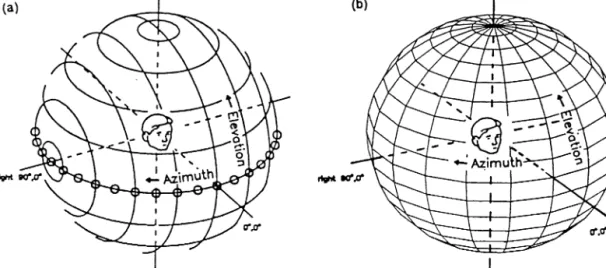
A two-dimensional, single pole spherical coordinate system was used to describe points on a unit sphere centered about the subject’s head. A point directly in front corresponds to zero azimuth and zero elevation. The azimuth coordinate (az) increases in a clockwise direction from the subject’s head and elevation (el) increases in an upwards direction (see Fig. 1). This coordinate system will be referred to as ‘hoop coordi-nates’ since it corresponds to the coordinates used in our laboratory by the automated robot arm in placing the auditory stimulus on an imaginary sphere surround-ing the subject. This coordinate system is commonly used in auditory localization literature and positions on the sphere are represented as the ordered pair (az, el). It should be noted that this particular choice of coordi-nate system restricts the analysis to data lying on the
Fig. 1. The double pole coordinate system (a) compared with the (single pole) hoop coordinate system (b).
sphere, and in particular, does not give a measure of distance (which would be the third dimension). One way in which this method could be used to display distance data would be to use surface color to indicate distance, however, this is not explored here.
Although, by convention, hoop coordinates are al-ways used in our software to describe positions in space, it is often mathematically more convenient to perform calculations in polar coordinates (u,f). To convert between the coordinates, the following formu-lae were used:
u=90−el f= −az
2.2. Mean direction
In order to calculate the mean direction of a set of points on the sphere, it is not sufficient to average the azimuth and elevation values since the hoop coordinate system is discontinuous. A simple averaging of points at hoop coordinates (0, 0) and (359, 0) would give the undesirable value of (179.5, 0).
Instead, the mean direction (u(,f( ) of a set of n data points Pi (=(ui,fi)) was computed by firstly finding
the Cartesian coordinates (also known as the direction cosines) (xi,yi,zi) using the formula (Fisher et al.,
1993):
xi=sinuicosfi, yi=sinuisinfi, zi=cosui
The vector sum of the unit vectors OPi (O is the
origin) is then computed:
Sx= % n i=1 xi, Sy=% n i−1 yi, Sz=% n i=1 zi
The mean direction has a resultant length of:
R=S2
x+S2y+S2z
Since our spherical coordinate system only allows unit length vectors, the resultant length can be used as a measure of dispersion (Wightman and Kistler, 1989).
R can range between 0 and n, with a large value corresponding to low dispersion, and small values cor-responding to increasingly uniform distributions of the data on the sphere.
For the direction cosines: (x¯,y¯,z¯)=(Sx/R,Sy/R,Sz/R)
These can be converted into polar coordinates using the following formulae:
u=arccos(z¯), f=arctan(y¯/x¯)
2.3. Kent distribution
Localization errors can be analyzed using the Kent distribution (Kent, 1982, Fisher et al., 1993)1which can
deal with asymmetric data. Using this method of mod-eling, no assumptions are made about the distribution of the data. The Kent distribution is a generalization of the Fisher distribution which assumes that the data is unimodal and has rotational symmetry. As can be seen in Fig. 2 (extracted from the same data set as Fig. 3), the top set of data points has a much wider variance in the azimuth direction thus leading to an ellipse shape (so is best described using the Kent distribution), whereas the bottom set of data is much more circular since the data is almost rotationally symmetric and can be described by a Fisher distribution.
1The 1987 edition of Fisher et al. had some errors in the sections detailing the computation of the Kent distributuion. The 1993 paper-back edition corrected these (some in the text and some in the errata). We have verified with the authors that there is a final minor mistake in Example 5.28, but such elliptical confidence cones are not used in our software. Instead, we use the standard deviation which is propor-tional in size to the elliptical confidence cone.
P.Leong,S.Carlile/Journal of Neuroscience Methods80 (1998) 191 – 200
194
The Kent distribution is described by the parameters
G, k and b, where G is a 3×3 matrix containing the three 3×1 column vectors (j1,j2,j3). j1 is the mean
direction of the distribution,j2is the direction in which the data density is the highest (major axis), andj3is the
direction of least data density (minor axis). It is most convenient to think of G as being the rotation matrix which best aligns the mean direction to the ‘north pole’ (i.e. (0, 0, 1) in Cartesian coordinates) of the sphere, with the principal components aligned with the (u,f) axes, the ‘principal components’ of a dataset being the set of M orthogonal vectors in that space that account for the maximum amount of variance in the data; found using principal component analysis — or the Karhunen – Loe`ve transform as it is otherwise known (see e.g. Jolliffe, 1986). The k parameter describes the degree of concentration of the data about the pole of the distribution, andb is an ovalness parameter which is small for circular data and increases as the data becomes more ovoid. Using the shape parameterskand
b, unimodal distributions, (k/b)]2, can be distin-guished from bimodal distributions, (k/b)B2.
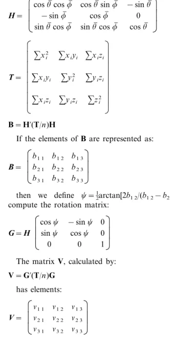
Estimates of the parameters of the Kent distribution (Fisher et al., 1993) can be computed forndata points (ui,fi) in polar coordinates (with corresponding direc-tion cosines (xi,yi,zi), resultant length R and mean
direction (u(,f( ) using the following formulae:
H=
Ã
Á
Ä
cosu( cosf( −sinf( sinu( cosf( cosu( sinf( cosf( sinu( cosf( −sinu( 0 cosu(Ã
Â
Å
T=Ã
Ã
Ã
Ã
Ã
Á
Ä
%x2 i %xiyi %xizi %xiyi %y2 i %yizi %xizi %yizi %z2 iÃ
Ã
Ã
Ã
Ã
Â
Å
B=H%(T/n)HIf the elements of B are represented as:
B=
Ã
Á
Ä
b1 1 b2 1 b3 1 b1 2 b2 2 b3 2 b1 3 b2 3 b3 3Ã
Â
Å
then we define c=1 2arctan[2b1 2/(b1 2−b2 2)] andcompute the rotation matrix:
G=H
Ã
Á
Ä
cosc sinc 0 −sinc cosc 0 0 0 1Ã
Â
Å
The matrix V, calculated by:
V=G%(T/n)G has elements: V=
Ã
Á
Ä
n1 1 n2 1 n3 1 n1 2 n2 2 n3 2 n1 3 n2 3 n3 3Ã
Â
Å
and if we define Q=n1 1−n2 2, using this and the
resultant length, we can calculate the shape parameters:
k= 1 2−2R−Q+ 1 2−2R+Q b=1 2
1 2−2R−Q− 1 2−2R+QThe parameters (G,k,b) describe the Kent distribution.
The Kent distribution can be used to determine whether a sample comes from a Fisher distribution as opposed to a Kent distribution using the following test statistic:
K=n(
1
2k)2I1/2(k)Q2
I5/2(k)
where I1/2(k) and I5/2(k) are modified Bessel
func-tions of the first kind. The hypothesis that the data comes from a Fisher distribution rather than a Kent distribution is rejected at the 100a% level if K\− Fig. 2. This figure shows two data sets which are shown as ‘’ (on
top) and ‘×’ (on bottom). The ‘×’ data is rotationally symmetric and follow a Fisher distribution (notice how the ellipse fitted to the data is circular). The ‘’ data is better modeled by the more general Kent distribution. The Kent distribution need not be rotationally symmetric and the major and minor axes of the ellipses drawn are aligned with the directions of greatest variance in the data.
Fig. 3. Spherical plot showing major and minor axes of the data variance obtained using the Kent distribution.
2 loga. For the example shown in Fig. 2, K=9.1 for the top (Kent) example and K=0.4 for the bottom (Fisher) example.
In order to obtain the ellipses displayed in Fig. 2 and Fig. 3, the data were first rotated using the Gmatrix, i.e.:
Ã
Á
Ä
xi% yi% z%iÃ
Â
Å
= GÃ
Á
Ä
xi yi ziÃ
Â
Å
This procedure aligns the principal components of the data with the azimuth and elevation axes, centered about the pole. The standard deviations along the axes are then calculated and an ellipse about the North pole with major and minor axes one standard deviation in size is computed. The ellipse is then rotated back to the mean position using theGmatrix to produce the plot-ting coordinates of an ellipse centered about the mean direction with major and minor axes in the principal directions of data variance.
2.4. Data collection
The aim of these types of experiments is to examine the accuracy with which a subject can determine the location of an auditory target or sound source. In our laboratory the target is placed randomly on the surface of an imaginary sphere (1 m radius) centered on the subject’s head using a computer controlled robot arm (see Carlile et al., 1996). The experiment is carried out in a darkened anechoic chamber to avoid extraneous acoustic and visual cues to target location. Following a short (150 ms) auditory stimulus, the subject is asked to turn to face the source of the sound and point to it with their nose. The position of the head is determined using an electromagnetic tracking device which provides az-imuth, elevation and roll as well as the translational position of the head (Polhemus, Isotrack). Following appropriate training (Carlile et al., 1996) this provides a reliable and objective measure of the perceived location of the sound. Overall localization accuracy and the types of mislocalizations evident under different
listen-P.Leong,S.Carlile/Journal of Neuroscience Methods80 (1998) 191 – 200
196
ing conditions and with different auditory targets can be used to probe localization processing.
2.5. Data manipulation
Although the extraction of data is a relatively trivial task, we have found that a large percentage of our previous code involved data manipulation. The simple interfaces, along with a small set of routines to sort, select and extract the data have considerably reduced the complexity of the scripts. As illustrated in Section 3, very small programs using this library are capable of implementing complicated procedures.
2.6. Library interface routines
In this section, the Spak routines available to the user are described. Conventions that are followed in Spak are that all data selection routines have an ‘ –ld’ (local-ization data) suffix, all spherical routines (statistical and plotting) have a ‘ –sp’ (spherical) suffix, and all conver-sion routines have a ‘2’ in them (for example, cart2hp
converts from Cartesian to hoop coordinates. For all of the main library routines (those that have ‘ –ld’ or ‘–sp’ suffixes), coordinates are expressed in hoop coordinates (as described above).
The localization data are assumed to be arranged as ann×4 matrix where n is the number of points in the data set and the four columns correspond to source azimuth, source elevation, and the azimuth and eleva-tion of the localizaeleva-tion estimate, respectively. Typically, data is extracted and processed one record at a time, where a record is the k×4 matrix representing all recordings from a given source location (i.e. all vectors in the matrix have identical first and second columns). A summary of the commands available in Spak is given in Table 1. A very small set of flexible library routines provides great utility.
3. Results
In this section, we provide examples of the types of visualizations possible using Spak. A feature of this software is that very few lines of code are required to produce visualizations of auditory localization data. All of the code used to generate the plots in Figs. 3 – 5 are given in Appendix A.
3.1. Front–back confusion plots
There are basically two different types of auditory localization errors. The first type, called ‘local errors’, are those where the subjects perceive the location to be within a few tens of degrees of the actual location. The second type, where the subject correctly identifies the
azimuth angle of the target with respect to the median plane but makes an error in the hemisphere that the sound is judged to be located. These are called ‘front – back confusion errors’, as, for example, where a sound is located 10 degrees to the left of the frontal median plane and the subject perceives the location to be say 15 degrees left of the rearward median plane. In our applications, the latter type of error is relatively infre-quent (at most a few percent of the total number of localization judgments in a given study), and results in a weakly bimodal data set (the Kent distribution analy-sis routines also check and report on whether the data is unimodal or bimodal). One approach is to extract the front – back confusion data (e.g. Makous and Middle-brooks, 1990) and analyze these data separately (see Carlile, 1996, for details). The set of routines described here provide a filter to achieve this (rfb –sp( )). Other methods used for dealing with front – back confusions include resolving front – back confusions by reflecting the perceived location about the interaural axis before computing descriptive statistics (e.g. Wightman and Kistler, 1989) or avoid summary statistics altogether by showing all of the data graphically (e.g. Kistler and Wightman, 1992). In the latter two cases, routines from
Table 1
Summary of the routines available in Spak Routine Description
Returns all of the records bound within the sel –ld( )
rectangle defined by two locations on the sphere
Arranges the data in a canonical form (in-sort –ld( )
creasing in elevation with the azimuth in-creasing within the same elevation) so that all data from the same source location are adjacent
next –ld( ) Returns the next record as well as a copy of the matrix with the chosen record removed. The truncated matrix can be used as the next argument to next –ld( ) to iterate through all of the data
get –ld( ) Returns the data associated with a particular location
closest –ld( ) Returns the record with the closest match (Euclidean distance) to a particular location rfb –ld( ) Remove front – back confusions associated
with localization data
amov –sp( ) Translate the points specified by the second parameter by the amount specified in the first parameter
mean –sp( ) Computes the centroid of a record median –sp( ) Computes the median of a record kent –sp( ) Compute the Kent distribution parameters
of a record draw –sp( ) Draw a sphere
Draw a polygon which connects the points line –sp( )
given as input arguments
plot –sp( ) Draw dots at each point given in the input matrix
Fig. 4. Plot showing front – back confusion information on anX–Yplot.
the Spak library could be employed along with stan-dard MATLAB functions to filter the data appropri-ately before plotting.
The front – back confusions can be visualized using plots of Fig. 4 (Makous and Middlebrooks, 1990), the file ‘testfb.m’ in Appendix A showing the code used to produce the plot. The code uses the sample
psycho-physical data contained in the file ‘bigloc.asc’ and the processing shows the results of extracting out the front – back confusion data in the data set and plotting these on an X–Y plot where elevation has been col-lapsed. The extracted data is shown by the filled circles and the remaining data is plotted as small crosses. Lines 6 and 9 extract the local errors and the front – back confusion data, respectively, which are plotted on lines 12 and 14. The other lines of code are used to load the data and to annotate the plot, and are standard MATLAB commands.
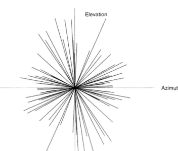
3.2. Directional line plots
Directional line plots can be used to visualize the directions of the principal components of the errors. The file ‘testdl.m’ in Appendix A (line 24) produces the plot of Fig. 5. The kent –sp( ) routine is called to compute the direction of the principal components (line 43), and then a line through the origin, which points in the direction of the first principal component and has length proportional to the standard deviation is com-puted using the amov –sp( ) routine (line 46) and plot-ted on line 47. Lines 38 – 40 and 50 – 51 perform a typical loop which iterates through all the data, one location at a time, and this type of loop is explained in greater detail in the next section.
Fig. 5. Directional line plots which show the directions of principal components of the data.
P.Leong,S.Carlile/Journal of Neuroscience Methods80 (1998) 191 – 200
198
On the resulting plot, if the errors are aligned with the coordinate system (as has been generally assumed in previous analyses), they will appear predominantly aligned with the vertical and horizontal axes, but in the case of the example in Fig. 5, this is clearly not the case.
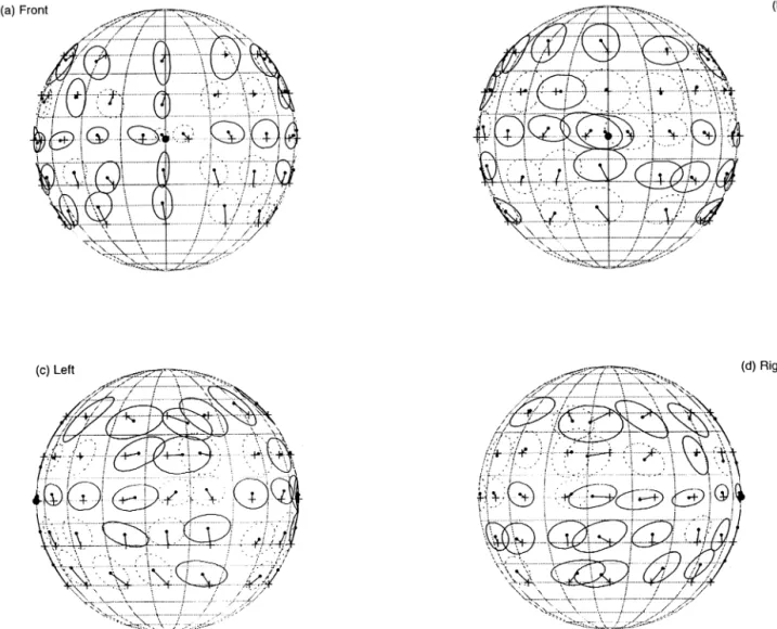
3.3. Spherical plots showing kent distribution
As a final example of the analysis and visualization possible using Spak, the MATLAB program which is shown in file ‘testkent.m’ of Appendix A is described in this section, producing the plot shown in Fig. 3. The program analyses each record using the kent –sp( ) rou-tine, and makes an ellipse centered around the centroid (i.e. the mean direction) of the measured results. A line is drawn between the centroid and the source location, and an ellipse with major and minor axes aligned with the principal components and with a size of one stan-dard deviation on each axis is drawn. If the data fits a Fisher distribution (i.e. it is rotationally symmetric in nature), this ellipse is drawn with a dotted line, other-wise, it must be a Kent distribution and it is drawn in a solid line.
On line 57, the matrix which describes the experimen-tal data is loaded. This is typical of the data resulting from a series of psychophysical experiments. The sub-routine akent( ) is called with arguments describing the location of the data of interest, and all of the processing is done in this routine. Note that, to do the ‘back’ plot of Fig. 3, akent( ) needs to be called twice (lines 67 and 68) to account for the fact that our coordinate system is discontinuous for this projection and we must therefore do the left and then the right projections separately. The akent( ) routine, which starts on line 76, begins by using sel –ld( ) to remove the data which will not be used for a particular projection. The data is then sorted to put it into a canonical form (line 81). Each record is then extracted using next –ld( ) (lines 86 and 98) which puts the record in ‘dat’ and the truncated data set in ‘sloc’.
The routine kent –sp( ) does all of the statistical work used in this example. This routine is called with the experimental data only (extracted using the MATLAB expression dat(:,[3 4])), and returns G, kappa, beta, q, ellz, ell, ln and isk. G, kappa, beta and q correspond to the Kent parameters G, k, b and Q described earlier, the two element vector ellz contains the sizes of one standard deviation along the principal components, ell contains a vector which if joined together forms an ellipse of size one standard deviation, and with the major and minor axes aligned with the principal direc-tions of the data errors, ln contains a vector of points making a line from the source location to the centroid, and isk being a boolean flag which is set if the data comes from a Kent distribution and zero if it is Fisherian.
On line 60, the output is set to be in landscape mode, and the current figure is cleared on line 61. Line 63 indicates that we wish to make 4 plots ar-ranged in a 2×2 grid, and the first graph is selected. The akent( ) routine is then called which will draw a sphere and plot the data on the first graph. The above procedure is repeated for the back, left and right plots.
The akent( ) routine firstly draws a sphere if dosp is set (line 82 – 84). The condition is required to avoid drawing two spheres when akent( ) is called twice for the same projection on lines 67 – 68. The view is then changed to that the location specified in the vcoord parameter becomes the center of that projection. Since the coordinates are assumed to be in hoop coordi-nates, they must first be converted to Cartesian coor-dinates for the MATLAB view( ) function.
Depending on the value of isk, ecol can be set to different line styles in lines 90 – 94. On line 95, a dot is drawn at the centroid of the data. A line is drawn from the source location to the centroid on line 96, and the ellipse is drawn with plotting parameter ecol on line 97.
The size of the ellipses in plots thus generated gives a good summary of auditory localization perfor-mance; the shape gives indications as to the relative contributions of the principal components; the orien-tation of the ellipse shows the alignment of the direc-tions of greatest variance and the lines from the source locations to the centroid give an indication of the absolute errors of an auditory localization trial. We have found that this type of plot gives a very good summary of the performance of an experiment in auditory localization.
4. Discussion
This paper documents the implementation of routines for data management, visualization and the statistical description of spherical data. In an effort to maximize the utility of these routines we have a exploited a very widely used data visualization and analysis package (MATLAB). The data management features of this package facilitate the efficient manipulation of large amounts of spherical data (\104 data points). Data can be sorted and that associated with particular loca-tions, or a range of locations can be extracted. Consid-erable effort has gone into implementing routines that represent a single functional step to provide the widest range of utility for each routine. Complex analytical sequences can be assembled with just a few lines of script.
A consistent set of coordinate conversion routines allows seamless movement from the popular single pole description of spatial location used in auditory research
to spherical coordinates and also to the Matlab plot-ting coordinates. The coordinates conversion routines are integrated into plotting routines so that the user only has to operate in the ‘native’ single pole descrip-tions of spatial location. The visualization routines exploit the three-dimensional plotting capabilities of MATLAB and could be integrated into an interactive user interface that is also available with MATLAB. Although these routines have been originally written to facilitate the analysis of auditory localization data they are sufficiently generalized to be applied to any spherical data set. At most, a user may have to write small MATLAB script to convert the coordinate sys-tem used by their own data to a spherical coordinate system to make available the full functionality of this package.
As illustrated using the sample data set in Fig. 2, the distributions of localization errors for many spa-tial locations are not rotationally symmetrical and are better described using an ellipse. The axes of the el-lipse correspond to the first two principal components and, for a significant fraction of the data, the axes are not aligned with the axis of the coordinate sphere. This is most clearly seen in the directional line plots (Fig. 5) introduced in this paper. Summary statistics computed using the directions of the principal compo-nents can lead to more revealing information than either analyzing the azimuth and elevation axes inde-pendently, or combining them and assuming rota-tional symmetry. Similar kinds of spherical analysis of the underlying cues to sound location will indicate to what extent the characteristics of the error distribu-tions are dependent on the nature of the spatially dependent changes in the cues to locations.
In the previous studies of auditory localization pro-cessing at least two coordinate systems have been used in describing spatial location (single pole and double pole). A lack of a standard method for repre-sentation and analysis has resulted in enormous difficulties in comparing the results of different studies in this area. It is hoped that researchers will be able to use this package to analyze and display results from their own experiments and hence facilitate a greater uniformity in the presentation and analysis of data in this and related research fields.
Acknowledgements
This work was supported by the Australian Re-search Council (AC9330318) and a University of Syd-ney Research grant. The authors would like to thank Dr Markus Schenkel for reviewing an earlier draft of this paper.
P.Leong,S.Carlile/Journal of Neuroscience Methods80 (1998) 191 – 200
200
References
Carlile S. Virtual Auditory Space: Generation and Applications, Landes, Austin, 1996.
Carlile S, Leong P, Hyams S, Pralong D. The nature and distribution of errors in the localization of sounds by humans. Hear Res 1997;114:179 – 96.
Fisher NI, Lewis T, Embleton BJJ. Statistical Analysis of Spherical Data. Cambridge University Press, Cambridge, 1993, paperback edition (with errata).
Jolliffe, I.T. Principal Component Analysis. Springer-Verlag, New York, 1986.
Kent JT. The Fisher – Bingham distribution on the sphere. J R Statist Soc B 1982;44:71 – 80.
Kistler DJ, Wightman FL. A model of head-related transfer functions based on principal components analysis and minimum phase reconstruction. J Acoust Soc Am 1992;91:1637 – 47.
Makous J, Middlebrooks JC. Two-dimensional sound localization by human listeners. J Acoust Soc Am 1990;87:2188 – 200.
Oldfield WR, Parker SPA. Acuity of sound localization: a topography of auditory space I. Normal hearing conditions. Perception 1984;13:581 – 600.
Tufte ER. Envisioning Information. Graphic Press, Cheshire, CT, 1990. Wightman FL, Kistler DJ. Headphone simulation of free field listening. II: Psychophysical validation. J Acoust Soc Am 1989;85:868 – 78.