A hybrid DE–PS algorithm for load frequency control under deregulated power system with UPFC and RFB

(1)

ELECTRICAL ENGINEERING

A hybrid DE–PS algorithm for load frequency

control under deregulated power system

with UPFC and RFB

Rabindra Kumar Sahu

*

_{, Tulasichandra Sekhar Gorripotu, Sidhartha Panda}

Department of Electrical Engineering, Veer Surendra Sai University of Technology (VSSUT), Burla 768018, Odisha, India Received 28 November 2014; revised 20 February 2015; accepted 3 March 2015

Available online 25 April 2015

KEYWORDS

Load Frequency Control (LFC);

Generation Rate Constraint (GRC);

Governor Dead Band (GDB);

Differential Evolution (DE); Uniﬁed Power Flow Controller (UPFC); Redox Flow Battery (RFB)

Abstract In this paper, a Modified Integral Derivative (MID) controller is proposed for Load Frequency Control (LFC) of multi-area multi-source power system in deregulated environment. The multi-source power system is having different sources of power generation such as thermal, hydro, wind and diesel generating units considering boiler dynamics for thermal plants, Generation Rate Constraint (GRC) and Governor Dead Band (GDB) non-linearity. The superior-ity of proposed hybrid Differential Evolution and Pattern Search (hDE-PS) optimized MID con-troller over GA and DE techniques is demonstrated. Further, the effectiveness of proposed hDE-PS optimized MID controller over Integral (I) and Integral Derivative (ID) controller is verified. Then, to further improve the system performance, Unified Power Flow Controller (UPFC) is placed in the tie-line and Redox Flow Batteries (RFBs) are considered in the first area. The performance of proposed approach is evaluated at all possible power transactions that take place in a deregulated power market.

2015 Faculty of Engineering, Ain Shams University. Production and hosting by Elsevier B.V. This is an open access article under the CC BY-NC-ND license (http://creativecommons.org/licenses/by-nc-nd/4.0/).

1. Introduction

The main objective of power system control is to maintain con-tinuous supply of power with an acceptable quality, to all the

consumers in the system. The system will be in equilibrium, when there is a balance between the power demand and the power generated. There are two basic control mechanisms used to achieve reactive power balance (acceptable voltage proﬁle) and real power balance (acceptable frequency values). In an interconnected power system a sudden load change in one area causes the deviation of frequency of all the areas. This change in frequency is to be corrected by Load Frequency Control (LFC) [1,2]. Nevertheless, the users of the electric power change the loads randomly and momentarily. It is impossible to maintain the balances between generation and load without control. So, a control system is essential to cancel the effects of the random load changes and to keep the frequency at the standard value[3].

* Corresponding author. Tel.: +91 9439702316.

E-mail addresses:[email protected](R.K. Sahu),gtchsekhar@ gmail.com (T.S. Gorripotu), [email protected] (S. Panda).

Peer review under responsibility of Ain Shams University.

Production and hosting by Elsevier

Ain Shams University

Ain Shams Engineering Journal

www.elsevier.com/locate/asej www.sciencedirect.com

http://dx.doi.org/10.1016/j.asej.2015.03.011

2090-44792015 Faculty of Engineering, Ain Shams University. Production and hosting by Elsevier B.V. This is an open access article under the CC BY-NC-ND license (http://creativecommons.org/licenses/by-nc-nd/4.0/).

(2)

In a traditional power system conﬁguration, generation, transmission and distribution of an electrical power are owned by a single entity called as Vertically Integrated Utility (VIU), which supplies power to the customers at regulated tariff. In an open energy market, Generating Companies (GENCOs) may or may not participate in the LFC task as they are indepen-dent power utilities. On the other hand, Distribution Companies (DISCOs) may contract with GENCOs or Independent Power Producers (IPPs) for the transaction of power in different areas[4]. Thus, in deregulated environment, control is greatly decentralized and Independent System Operators (ISOs) are responsible for maintaining the system fre-quency and tie-line power ﬂows[4,5].

The researchers in the world over are trying to propose sev-eral strategies for LFC of power systems under deregulated environment in order to maintain the system frequency and tie-line ﬂow at their scheduled values during normal operation and also during small perturbations. Recently, Parmar et al.

[6]have studied the multi-source power generation in deregu-lated power environment using optimal output feedback con-troller. Debbarma et al.[7]have proposed AGC of multi-area thermal power systems under deregulated power environment considering reheat turbines and GRC, where the fractional order PID controller parameters are optimized employing Bacterial Foraging (BF) optimization technique and the results are compared with classical controller to show its superiority. Demiroren and Zeynelgil[8]have suggested AGC in three area power system after deregulation and used GA technique to ﬁnd the optimal integral gains and bias factors. A four area power system in a deregulated environment has been examined in[9]. Hybrid particle swarm optimization is used to obtain optimal gain of PID controller. However, in the above literatures the

effect of physical constraints such as Generation Rate Constraint (GRC) and Governor Dead Band (GDB) nonlinear-ity is not examined which needs further comprehensive study.

Several classical controllers structures such as Integral (I), Proportional–Integral (PI), Integral–Derivative (ID), Proportional–Integral–Derivative (PID) and Integral–Double Derivative (IDD) have been explored in[10]. Tan and Zhang

[11] have been proposed Two Degree of Freedom (TDF) Internal Model Control (IMC) method to tune decentralized PID type load frequency controllers for multi-area power sys-tems in deregulated power environments. Liu et al.[12]have been suggested optimal Load Frequency Control (LFC) under restructured power systems with different market structures. It is found from the literature survey that, most of the work is limited to reheat thermal plants, hydro plants and relatively lesser attention has been devoted to wind, diesel generating units. Due to insufﬁcient power generation and environmental degradation issues, it is necessary to make use of wind energy in favorable locations[13]. Keeping in view the present power scenario, combination of multisource power generation with their corresponding participation factors is considered for the present study.

Flexible AC Transmission Systems (FACTS) controllers play a crucial role to control the power flow in an intercon-nected power system. Several studies have explored the poten-tial of using FACTS devices for better power system control since it provides more flexibility. Unified Power Flow Controller (UPFC) is one of the most versatile FACTS con-trollers which is connected in series with the transmission line or in a tie-line to improve the damping of oscillations [14]. Redox Flow Batteries (RFBs) are an active power source which can be essential not only as a fast energy compensation

Nomenclature

apf ACEparticipation factor

a12 PR1=PR2

ACEi area control error of areai

Bi Frequency bias parameter of areai(p.u.MW/Hz)

cpfmn contract participation factor betweenmthGENCO

andnthDISCO

CR crossover probability

DPM DISCOparticipation matrix

F nominal system frequency (Hz)

FC step size

G number of generation

GDB governor dead band

GRC generation rate constraint i subscript referred to areai(1, 2) Kdiesel gain of diesel unit

Kri steam turbine reheat constant of areai

KRFB gain of Redox Flow Battery

KPSi power system gain of areai(Hz/p.u.MW)

NP number of population size

PRi rated power of areai(MW)

tsim simulation time (s)

Tri steam turbine reheat time constant of areai(s)

TGi speed Governor time constant for thermal unit of

areai(s)

TGHi hydro turbine speed governor main servo time

constant of areai(s)

TPSi power system time constant of areai(s)

TRFB time constant of Redox Flow Battery (s)

TRHi hydro turbine speed governor transient droop time

constant of areai(s)

TRSi hydro turbine speed governor reset time of areai

(s)

TTi steam turbine time constant of areai(s)

TUPFC time constant of UPFC (s)

TWi nominal starting time of water in penstock of area

i(s)

T12 synchronizing coefﬁcient between areas 1 and 2 (p.u.)

DFi incremental change in frequency of areai(Hz)

DPDi incremental step load change of areai

DPTie incremental change in tie-line power between areas

1 and 2 (p.u.)

DPactual_Tie_;12 change in actual tie-line power (p.u.MW)

DPerror_Tie_;12 change in tie-line power error (p.u.MW)

DPscheduled_Tie_;12 change in scheduled steady state tie-line power (p.u.MW)

(3)

device for power consumptions of large loads, but also as a sta-bilizer of frequency oscillations[15–17]. The RFB will, in addi-tion to load compensating, have other applicaaddi-tions such as power quality maintenance for decentralized power supplies. But, due to the economical reasons it is not possible to place RFB in all the areas. When UPFC and RFB are present in the system, they should act in a coordinated manner so as to control the network conditions in a very fast and economical manner.

It is obvious from the literature survey that the performance of the power system depends on the controller structure and the techniques employed to optimize the controller parameters. Hence, proposing and implementing new controller approaches using high performance heuristic optimization algorithms to real world problems are always welcome. For any meta-heuris-tic algorithm, a good balance between exploitation and explo-ration during search process should be maintained to achieve good performance. DE being a global optimizing method is designed to explore the search space and most likely gives an optimal/near-optimal solution if used alone. On the other hand, local optimizing methods like Pattern Search (PS) are designed to exploit a local area[18], but they are usually not good at exploring wide area and hence not applied alone for global optimization. Due to their respective strength and weakness, there is motivation for the hybridization of DE and PS.

In view of the above, a maiden attempt has been made in this paper to apply a hybrid DE–PS optimization technique to tune MID controller for the LFC of multi-area multi-source power systems under deregulated environment with the consideration of boiler dynamics for thermal plants, Generation Rate Constraint (GRC) and Governor Dead Band (GDB) non-lin-earity. The superiority of the proposed approach is shown by comparing the results with GA and DE techniques for the same power system. Additionally the dynamic performance of the sys-tem is investigated with integral and ID controllers. Further, UPFC is employed in series with the tie-line in coordination with RFB to improve the dynamic performance of the system. The effectiveness of the proposed controllers with the change in sys-tem parameters or loading conditions is assessed for the syssys-tem under study. It is observed that the proposed controllers are robust and need not be retuned when the system is subjected to wide variation in system parameter and loading condition. Finally, demonstrating the ability of the proposed approach under random load perturbation has been investigated.

2. Material and method

2.1. System under study

Load Frequency Control (LFC) provides the control only dur-ing normal changes in load which are small and slow. So the nonlinear equations which describe the dynamic behavior of the system can be linearized around an operating point during these small load changes and a linear incremental model can be used for the analysis thus making the analysis simpler.

A realistic network of two-area six-unit power systems with different power generating units [19] considering the boiler dynamics for thermal plants, Generation Rate Constraint (GRC) and Governor Dead Band (GDB) non-linearity is shown in Fig. 1. Each area has a rating of 2000 MW with a nominal load of 1640 MW. Area-1 consists of reheat thermal,

hydro, wind power plants and two DISCOs namely DISCO1 and DISCO2. Area-2 comprises of reheat thermal, hydro, die-sel power plants and two DISCOs namely DISCO3 and DISCO4 as shown inFig. 1. The transfer function model of wind and diesel generating units is adopted from [13]. The transfer function model of wind turbine system with pitch con-trol is shown inFig. 1. The model consists of hydraulic pitch actuator, data fit pitch response and blade characteristics. The diesel unit is represented by a transfer function as shown inFig. 1. Each unit has its regulation parameter and participa-tion factor which decide the contribuparticipa-tion to the nominal load-ing, summation of participation factor of each control being equal to 1. Due to the presence of large thermal plants, their participation factor is generally large in the range of 50– 60%. The participation factors of hydrounits are about 30%. As, wind and diesel generating power generations are less, their participation is usually low which is about 10–15%[19]. In the present study, participation factors for thermal and hydro are assumed as 0.575 and 0.3 respectively. For wind and diesel same participation factors of 0.125 are assumed. The nominal parameters of the system under study are given inAppendix A. The boiler dynamics configuration is incorporated in thermal plants to generate steam under pressure. This model considers the long-term dynamics of fuel and steam flow on boiler drum pressure as well as combustion controls. The block diagram of boiler dynamics [19] configuration is shown in Fig. 2. Governor dead band is defined as the total amount of a con-tinued speed change within which there is no change in valve position. Steam turbine dead band is due to the backlash in the linkage connecting the servo piston to the camshaft. Much of this appears to occur in the rack and pinion used to rotate the camshaft that operates the control valves. Due to the governor dead band, an increase/decrease in speed can occur before the position of the valve changes. The speed gov-ernor dead band has a great effect on the dynamic perfor-mance of electric energy system. The backlash non-linearity tends to produce a continuous sinusoidal oscillation with a natural period of about 2 s. For this analysis, in this study backlash nonlinearity of 0.05% for the thermal system is con-sidered. In a power system, power generation can change only at a specified maximum rate known as Generation Rate Constraint (GRC). Presence of GRC will affect adversely the system performance in LFC studies. Hydropower plant gener-ating units are normally adjusted as the response is faster to raise/lower the power. Thermal power plants have rate restric-tions due to thermal stresses even though all units are expected to participate in primary frequency regulation. If wind and die-sel powers are available, the system performance improves with the inclusion of wind and diesel units. The improvement in the system response is due to the absence of physical con-straints for wind and diesel units and they can quickly pick up the additional load demand thus stabilizing the system more quickly. In the present study, a GRC of 3% per min is considered for thermal units. The GRCs for hydrounit are 270% per minute for raising generation and 360% per minute for lowering generation are considered[19,20].

2.2. LFC in restructured scenario

The conventional AGC schemes aim to attain optimal genera-tion allocagenera-tion to the generator units. However, under

(4)

deregulation, AGC is allowed to control the contract powers of IPPs (Independent Power Producers) rather than the out-puts of generation units. In deregulated environment, AGC adapts the market requirement with several kinds of the

bidding strategies in order to achieve the economic optimality. All IPPs participate in electricity power bidding and provide unit prices or the incremental cost curves. Hence, in a deregu-lated environment, the AGC is mostly rederegu-lated to the bidding Figure 1 MATLAB/Simulink model of two-area diverse source power system under restructured scenario.

(5)

adjustment, which is performed by the market competition based on the incremental cost curves. The contract participa-tion factors provide a compact yet precise way of summarizing contractual arrangements.

In restructured scenario, the GENCOs in one area may supply DISCOs in same area as well as DISCOs in other areas. The DISCOs have the freedom to purchase power from differ-ent GENCOs at competitive prices. The various combinations of contracts between DISCOs and GENCOs are analyzed by the concept of a DISCO Participation Matrix (DPM) [4,9]. The rows of a DPM correspond to GENCOs and columns rep-resent to DISCOs which contract power. The corresponding DPM for the system is as follows:

DPM¼ cpf11 cpf12 cpf13 cpf14 cpf21 cpf22 cpf23 cpf24 cpf31 cpf32 cpf33 cpf34 cpf41 cpf42 cpf43 cpf44 cpf51 cpf52 cpf53 cpf54 cpf61 cpf62 cpf63 cpf64 2 6 6 6 6 6 6 6 6 4 3 7 7 7 7 7 7 7 7 5 ð1Þ

wherecpfrepresents contract participation factor. Each entry in this matrix can be thought as a fraction of a total load con-tracted by a nth-DISCO (column) toward a mth-GENCO (row). The sum of all the entries in a column in this matrix is unity and mathematically it can be expressed as follows:

X6

m¼1

cpfmn¼1 ð2Þ

The scheduled steady state power ﬂow on the tie-line can be given as follows:

DPscheduled

Tie;12 ¼ ðDemand of DISCOs in area1 to GENCOs in area2Þ

ðDemand of DISCOs in area2 to GENCOs in area1Þ ð3Þ

Mathematically Eq.(3)can be deﬁned as follows:

DPscheduled Tie;12 ¼ X3 m¼1 X4 n¼3 cpfmnDPLn X6 m¼4 X2 n¼1 cpfmnDPLn ð4Þ

The actual tie-line power can be represented as follows:

DPactual Tie;12¼

2pT12

s ðDF1DF2Þ ð5Þ

The tie-line power error can now be expressed as follows:

DPerror Tie;12¼DP actual Tie;12DP scheduled Tie;12 ð6Þ DPerror

Tie;12 reduces to zero in the steady as the actual tie-line

power ﬂow reaches the scheduled power ﬂow. The generated power or contracted power supplied by the GENCOs is given as follows:

DPgm¼ X4

n¼1

cpfmnPLn ð7Þ

This error signal is used to generate the respective Area Control Error (ACE) signals during the traditional scenario as given below:

ACE1¼B1DF1þDPerrorTie;12 ð8Þ

ACE2¼B2DF2þDPerrorTie;21 ð9Þ

As there are three GENCOs in each area,ACEsignal has to be distributed among them in proportion to their participation in the LFC. Coefﬁcients that distributeACEto GENCOs are ter-med as ‘‘ACEParticipation Factors (apfs)’’. In a given control area, the sum of participation factors is equal to 1. Hence, apf11,apf12,apf13are considered asACEparticipation factor

in area-1 andapf21,apf22,apf23are in area-2. Participation

fac-tors for thermal and hydro are assumed as 0.575 and 0.3 respectively. For wind and diesel same participation factor of 0.125 is assumed.

2.3. Controller structure and Objective function

As the areas are assumed unequal, different Modiﬁed Integral Derivative (MID) controllers are considered for each generat-ing unit to minimize the frequency oscillations and to control the tie-line powers. The MID control scheme is shown in

Fig. 3. Design of MID controller requires determination of the two main parameters, integral time constant (KI) and

Derivative time constant (KDD).

The error inputs to the controllers are the respective area control errors (ACE) given by the following:

Figure 2 Block diagram of boiler dynamics conﬁguration.

(6)

e1ðtÞ ¼ACE1¼B1DF1þDPTie ð10Þ

e2ðtÞ ¼ACE2¼B2DF2þa12DPTie ð11Þ

MID controller usesACE1 as input in area-1 and ACE2 in

area-2. In area-1, the outputs of the MID controllers UTH1;UHY1 and UW1 are the control inputs of the thermal,

hydro and wind generating units respectively. In area-2, the outputs of the MID controllersUTH2,UHY2 andUD2 are the

control inputs of the power system. The integral and derivative gains of the MID controllers are represented asKI1, KI2, KI3, KI4, KI5, KI6, KDD1, KDD2, KDD3, KDD4, KDD5 and KDD6

respectively.

In the design of a modern heuristic optimization technique based controller, the objective function is first defined based on the desired specifications and constraints. Performance criteria usually considered in the control design are the Integral of Time multiplied Absolute Error (ITAE), Integral of Squared Error (ISE), Integral of Time multiplied Squared Error (ITSE) and Integral of Absolute Error (IAE). ITAE criterion reduces the settling time which cannot be achieved with IAE or ISE based tuning. ITAE criterion also reduces the peak overshoot. ITSE based controller provides large controller output for a sudden change in set point which is not advanta-geous from controller design point of view. It has been reported that ITAE is a better objective function in LFC stud-ies[21]. Therefore in this paper ITAE is used as objective func-tion to optimize the MID controller. Expression for the ITAE objective function is depicted in Eq.(12).

J¼ITAE¼

Z tsim

0

ðjDF1j þ jDF2j þ jDPTiejÞ tdt ð12Þ

In the above equations,DF1andDF2are the system frequency

deviations;DPTie is the incremental change in tie- line power;

tsim is the time range of simulation. The problem constraints

are the MID controller parameter bounds. Therefore, the design problem can be formulated as the following optimiza-tion problem.

MinimizeJ ð13Þ

Subject toKImin6KI6KImax;KDDmin6KDD6KDDmax ð14Þ

2.4. Modeling of UPFC in LFC

During the last decade, continuous and fast improvement of

power electronics technology has made Flexible AC

Transmission Systems (FACTS) a promising concept for power system applications. With the application of FACTS technology, power flow along transmission lines can be more flexibly controlled. The Unified Power Flow Controller (UPFC) is regarded as one of the most versatile devices in the FACTS family which has the capability to control of the power flow in the transmission line, improve the transient sta-bility, alleviate system oscillation and offer voltage support

[14]. The two-area power system with a UPFC as shown in

Fig. 4is considered in this study. The UPFC installed in series with a tie-line and provides damping of oscillations the tie-line power[22]. InFig. 4,Vse is the series voltage magnitude and

/se is the phase angle of series voltage. The shunt converter

injects controllable shunt voltage such that the real component of the current in the shunt branch balance the real power demanded by the series converter. It is clear fromFig. 4that, the complex power at the receiving-end of the line as follows:

PrealjQreactive¼VrIline¼Vr

ðVsþVseVrÞ jðXÞ ð15Þ where Vse¼ jVsej\ðds/seÞ ð16Þ

Solving Eq.(15), the real part as given below Preal¼ jVsjjVrj ðXÞ sinðdÞ þ jVsjjVsej ðXÞ sinðd/seÞ ¼P0ðdÞ þPseðd;/seÞ ð17Þ

The above equation, if Vse=0, it represents that the real

power is uncompensated system, whereas the UPFC series voltage magnitude can be controlled between 0 andVsemax,

and its phase angle ð/seÞ can be controlled between 0 and

360 at any power angle. The UPFC based controller can be represented in LFC as follows[23]: DPUPFCðsÞ ¼ 1 1þsTUPFC DFðsÞ ð18Þ

whereTUPFCis the time constant of UPFC. 2.5. Modeling of RFB in LFC

In an interconnected power system during the presence of small load perturbations and with optimized controller gains, the frequency deviations and tie-line power changes exist for long time durations. During such conditions the governor may not able to absorb the frequency deviations due to slow response and non-linearities present in the system model. Therefore, in order to reduce the frequency deviations and change in tie-line power, an active power source with quick response such as RFB can be expected to the most effective one[15,17]. The RFB is found to be superior over the other Figure 4 Two area interconnected power system with UPFC.

Generating Unit Load

Dual converter with Battery Energy Storage System

Charging _Discharging

(7)

energy storage devices like Superconducting Magnetic Energy Storage (SMES) because of its easy operating at normal tem-perature, very small losses during operating conditions and has long service life[16]. However, it will be difﬁcult to place RFB in each and every area in the interconnected power sys-tem due to the economical reasons. Since, RFB is capable of ensuring a very quick response[17],DF1is being used directly

as the input command value for load frequency control. The general block diagram of the RFB used for LFC in the inter-connected power system is shown inFig. 5 [24]. During very

small load duration battery charges and delivers the energy to the system during sudden load changes. The dual converter performs both rectiﬁer and inverter action. For sudden step load perturbation the change of output of a RFB is given as

[17] DPRFB¼ KRFB 1þsTRFB DF1 ð19Þ X0 X0 + [-1 0] X0 + [-1 0] X0 + [0 1] X0 + [0 -1]

Figure 6 Pattern search mesh points and the pattern.

Figure 7 Flowchart of proposed Hybrid Differential Evolution Pattern Search (hDE-PS) algorithm.

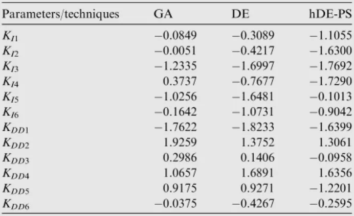
Table 1 Tuned MID controller parameters for different techniques under poolco based without UPFC and RFB.

Parameters/techniques GA DE hDE-PS KI1 0.0849 0.3089 1.1055 KI2 0.0051 0.4217 1.6300 KI3 1.2335 1.6997 1.7692 KI4 0.3737 0.7677 1.7290 KI5 1.0256 1.6481 0.1013 KI6 0.1642 1.0731 0.9042 KDD1 1.7622 1.8233 1.6399 KDD2 1.9259 1.3752 1.3061 KDD3 0.2986 0.1406 0.0958 KDD4 1.0657 1.6891 1.6356 KDD5 0.9175 0.9271 1.2201 KDD6 0.0375 0.4267 0.2595

(8)

whereKRFB is gain andTRFB is time constant of RFB in sec.

3. Hybrid differential evolution pattern search (hDE-PS) algorithm

To search the highly multimodal space, a two phase hybrid method known as hybrid Differential Evolution Pattern Search (hDE-PS) is employed. In this algorithm, DE is used for global exploration and the Pattern Search algorithm [18]

is employed for local search. The ﬁrst phase is explorative, employing a classical DE to identify promising areas of the search space. The best solution found by DE is then reﬁned using PS method during a subsequent exploitative phase. In order to establish the superiority of proposed hDE-PS approach, the results are compared with individual DE approach. Each of these algorithms is described below. 3.1. Differential evolution

Differential Evolution (DE) algorithm is a population-based stochastic optimization algorithm recently introduced [25]. Advantages of DE are: simplicity, efﬁciency and real coding, easy use and speediness. DE works with two populations; old generation and new generation of the same population. The size of the population is adjusted by the parameter NP.

The population consists of real valued vectors with dimension D that equals the number of design parameters/control vari-ables. The population is randomly initialized within the initial parameter bounds. The optimization process is conducted by means of three main operations: mutation, crossover and selec-tion. In each generation, individuals of the current population become target vectors. For each target vector, the mutation operation produces a mutant vector, by adding the weighted difference between two randomly chosen vectors to a third vec-tor. The crossover operation generates a new vector, called Table 2 Performance index for different techniques under

poolco based without UPFC and RFB.

Performance index GA DE hDE-PS

ITAE 2.4264 1.8503 1.6995

Settling TimeTS(s) DF1 38.91 32.74 28.84

DF2 38.93 33.56 29.52

DPTie 28.17 22.53 18.65 Peak over shoot DF1 0.0252 0.0138 0.0086

DF2 0.0032 0.0019 0.0027 DPTie 0.0024 0.0019 0.0017 0 5 10 15 20 25 30 -0.03 -0.02 -0.01 0 0.01 0.02 Time (sec) Δ F1 (Hz) (a)

GA: Without UPFC & RFB DE: Without UPFC & RFB hDE-PS: Without UPFC & RFB

0 5 10 15 20 25 30 -20 -15 -10 -5 0 5x 10 -3 Time (sec) Δ F2 (Hz) (b)

0 5 10 15 20 25 30 -15 -10 -5 0 x 10-3 Time (sec) Δ PTie (p.u.) (c)

Figure 8 Dynamic responses of the system under poolco based scenario without UPFC and RFB (a) frequency deviation of area-1 (b) frequency deviation of area-2 (c) tie-line power deviation.

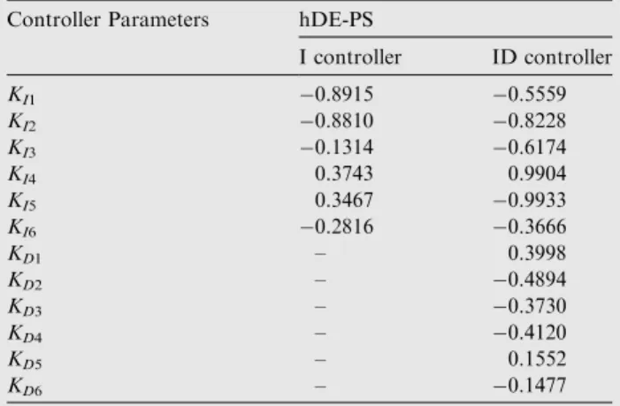
Table 3 Tuned I/ID controller parameters for hDE-PS technique under poolco based without UPFC and RFB.

Controller Parameters hDE-PS

I controller ID controller KI1 0.8915 0.5559 KI2 0.8810 0.8228 KI3 0.1314 0.6174 KI4 0.3743 0.9904 KI5 0.3467 0.9933 KI6 0.2816 0.3666 KD1 – 0.3998 KD2 – 0.4894 KD3 – 0.3730 KD4 – 0.4120 KD5 – 0.1552 KD6 – 0.1477

Table 4 Performance index for different controllers under poolco based without UPFC and RFB.

Parameters hDE-PS I controller ID controller Proposed MID controller ITAE 3.5887 2.8375 1.6995 TS(s) DF1 47.47 28.79 28.84 DF2 48.18 28.51 29.52 DPTie 40.45 21.47 18.65 Peak over shoot DF1 0.0102 0.0092 0.0086 DF2 0.0043 0.0036 0.0027 DPTie 0.0031 0.0022 0.0017

(9)

trial vector, by mixing the parameters of the mutant vector with those of the target vector. If the trial vector obtains a bet-ter ﬁtness value than the target vector, then the trial vector replaces the target vector in the next generation. The DE algo-rithm is explained in more detail in[26].

3.2. Pattern search

The Pattern Search (PS) optimization technique is a derivative free evolutionary algorithm suitable to solve a variety of opti-mization problems that lie outside the scope of the standard optimization methods. It is simple in concept, easy to imple-ment and computationally efficient. It possesses a flexible and well-balanced operator to enhance and adapt the global search and fine tune local search[18]. The PS algorithm com-putes a sequence of points that may or may not approach to the optimal point. The algorithm starts with a set of points called mesh, around the initial points. The initial points or cur-rent points are provided by the DE technique. The mesh is cre-ated by adding the current point to a scalar multiple of a set of vectors called a pattern. If a point in the mesh is having better objective function value, it becomes the current point at the next iteration[27].

The Pattern search begins at the initial point X0 that is given as a starting point by the DE algorithm. At the ﬁrst iter-ation, with a scalar = 1 called mesh size, the pattern vectors or

direction vectors are constructed as [0 1], [1 0], [1 0] and [01]. The direction vectors are added to the initial point X0 to compute the mesh points as X0 + [0 1], X0 + [1 0], X0 + [1 0] and X0 + [01] as shown in Fig. 6. The algo-rithm computes the objective function at the mesh points in the same order. The algorithm polls the mesh points by com-puting their objective function values until it ﬁnds one whose value is smaller than the objective function value of X0. Then the poll is said to be successful when the objective func-tion value decreases at some mesh point and the algorithm sets this point equal to X1. After a successful poll, the algorithm steps to iteration 2 and multiplies the current mesh size by 2. As the mesh size is increased by multiplying by a factor i.e. 2, this is called the expansion factor. So in 2nd iteration, the mesh points are: X1 + 2 * [0 1], X1 + 2 * [1 0], X1 + 2 * [1 0] and X1 + 2 * [01] and the process is repeated until stopping criteria is met. Now if in a particular iteration, none of the mesh points has a smaller objective func-tion value than the value at initial/current point at that itera-tion, the poll is said to be unsuccessful and same current point is used in the next iteration. Also, at the next iteration, the algorithm multiplies the current mesh size by 0.5, a con-traction factor, so that the mesh size at the next iteration is smaller and the process is repeated until stopping criteria is met. The ﬂow chart of proposed hybrid Pattern Search (PS) and DE approach is shown inFig. 7.

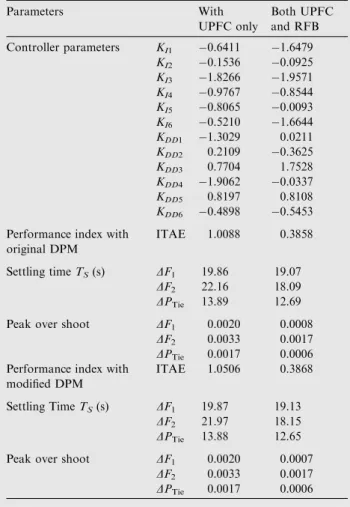
Table 5 Tuned controller parameters and performance index for poolco based transaction with UPFC and RFB.

Parameters With UPFC only Both UPFC and RFB Controller parameters KI1 0.6411 1.6479 KI2 0.1536 0.0925 KI3 1.8266 1.9571 KI4 0.9767 0.8544 KI5 0.8065 0.0093 KI6 0.5210 1.6644 KDD1 1.3029 0.0211 KDD2 0.2109 0.3625 KDD3 0.7704 1.7528 KDD4 1.9062 0.0337 KDD5 0.8197 0.8108 KDD6 0.4898 0.5453 Performance index with

original DPM

ITAE 1.0088 0.3858

Settling timeTS(s) DF1 19.86 19.07

DF2 22.16 18.09

DPTie 13.89 12.69 Peak over shoot DF1 0.0020 0.0008

DF2 0.0033 0.0017

DPTie 0.0017 0.0006 Performance index with

modiﬁed DPM

ITAE 1.0506 0.3868

Settling TimeTS(s) DF1 19.87 19.13

DF2 21.97 18.15

DPTie 13.88 12.65 Peak over shoot DF1 0.0020 0.0007

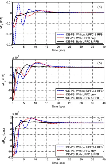
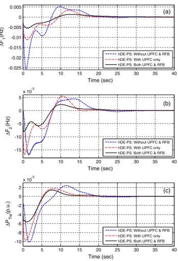
DF2 0.0033 0.0017 DPTie 0.0017 0.0006 0 5 10 15 20 25 30 35 40 -0.03 -0.02 -0.01 0 0.01 Time (sec) Δ F1 (H z ) (a)

hDE-PS: Without UPFC & RFB hDE-PS: With UPFC only hDE-PS: Both UPFC & RFB

0 5 10 15 20 25 30 35 40 -20 -15 -10 -5 0 x 10-3 Time (sec) Δ F2 (H z ) (b)

0 5 10 15 20 25 30 35 40 -12 -10 -8 -6 -4 -2 0 2x 10 -3 Time (sec) Δ PTi e ( p .u .) (c)

Figure 9 Dynamic responses of the system under poolco based scenario (a) frequency deviation of area-1 (b) frequency deviation of area-2 (c) tie-line power deviation.

(10)

4. Results and discussions

4.1. Design of proposed hybrid DE–PS optimized MID controller

The model of the system under study shown inFig. 1is devel-oped in MATLAB/SIMULINK environment and hybrid DE–PS program is written (in .mfile). Initially, dissimilar MID controllers are considered for each generating unit with-out considering the UPFC and RFB under poolco based transaction. The control gains of MID controller are chosen in the range [2, 2]. The developed model is simulated in a separate program (by .mfile using initial population/controller parameters) considering a 1% step load change (1% of nom-inal load i.e. 16.4 MW) in area-1. The objective function is calculated in the .mfile and used in the optimization algo-rithm. In the present study, a population size of NP= 40,

generation numberG= 30, step sizeFC= 0.2 and crossover probability of CR= 0.6 have been used [26]. One more important point that more or less affects the optimal solution is the range for unknowns. For the very ﬁrst execution of the program, wider solution space can be given, and after getting

the solution, one can shorten the solution space nearer to the values obtained in the previous iterations. Simulations were conducted on an Intel, Core i-5 CPU of 2.5 GHz,

8 GB, 64-bit processor computer in the MATLAB

7.10.0.499 (R2010a) environment. The optimization process was repeated 20 times for DE, PS and hDE-PS algorithm. The maximum number of iteration is set to 30 for individual DE and PS techniques. In hDE-PS approach, DE technique is applied for 20 iterations and PS is then employed for 10 iter-ations to fine tune the best solution provided by DE. PS is executed with a mesh size of 1, mesh expansion factor of 2 and mesh contraction factor of 0.5. The maximum number of objective function evaluations is set to 10. The best final solution corresponding to the minimum fitness values obtained among the 20 runs is chosen as controller parame-ters. The best final solution obtained in the 20 runs is chosen as controller parameters. For the implementation of GA, normal geometric selection, arithmetic crossover and nonuniform mutation are employed in the present study. A population size of 40 and maximum generation of 30 is employed in the present paper. A detailed description about GA parameters employed in the present paper can be found in reference[8].

4.2. Poolco based transaction

In this scenario DISCOs have contract with GENCOs of the same area. It is assumed that the load disturbance occurs only

0 5 10 15 20 25 30 35 40 -0.03 -0.02 -0.01 0 0.01 Time (sec) Δ F1 (Hz) (a)

0 5 10 15 20 25 30 35 40 -20 -15 -10 -5 0 x 10-3 Time (sec) Δ F2 (Hz) (b)

0 5 10 15 20 25 30 35 40 -12 -10 -8 -6 -4 -2 0 2 x 10-3 Time (sec) Δ PTie (p.u.) (c)

Figure 10 Dynamic responses of the system for poolco based scenario under changed contract participation factor (a) frequency deviation of area-1 (b) frequency deviation of area-2 (c) tie-line power deviation.

Table 6 Tuned MID controller parameters for bilateral based transaction.

Parameters Without UPFC and RFB

With UPFC only

Both UPFC and RFB KI1 1.3695 0.3991 1.8508 KI2 0.0009 0.1642 0.2280 KI3 0.6181 1.7254 1.7830 KI4 0.2876 0.9905 0.0836 KI5 1.8029 1.1901 0.9467 KI6 0.3662 1.6529 0.9800 KDD1 0.1873 0.3007 0.0697 KDD2 1.7571 0.4249 0.2910 KDD3 0.0644 1.1422 1.0465 KDD4 0.4916 0.0797 0.5740 KDD5 1.6104 1.9567 1.0594 KDD6 0.7602 0.0403 0.2104

Table 7 Performance index values under bilateral based transaction.

Parameters Without UPFC and RFB With UPFC only Both UPFC and RFB ITAE 2.0231 1.0331 0.5033 TS(s) DF1 31.00 22.81 20.15 DF2 38.13 21.72 18.58 DPTie 32.82 13.13 14.22 Peak over shoot DF1 0.0102 0.0017 0.0010 DF2 0.0039 0.0028 0.0016 DPTie 0.0028 0.0013 0.0009

(11)

in area-1. There is 0.005 (pu MW) load disturbance in DISCO1 and DISCO2, i.e. DPL1¼0:005 (pu MW), DPL2¼0:005 (pu

MW),DPL3¼DPL4¼0 (pu MW) as a result of the total load

disturbance in area-1 i.e.DPD1¼0:01 (pu MW). A particular

case of Poolco based contracts between DISCOs and available GENCOs is simulated based on the following DPM:

DPM¼ 0:5 0:5 0 0 0:3 0:3 0 0 0:2 0:2 0 0 0 0 0 0 0 0 0 0 0 0 0 0 2 6 6 6 6 6 6 6 6 4 3 7 7 7 7 7 7 7 7 5 ð20Þ

In the above case, DISCO3 and DISCO4 do not demand power from any GENCOs, and hence the corresponding contract participation factors are zero. Accordingly, theACE participation of GENCOs are: apf11=apf21= 0.575, apf12=apf22=0.3, apf13=apf23= 0.125. The scheduled

tie-line power in this case is zero.

In the steady state, generation of a GENCO must match the demand of DISCOs in contract with it. The desired gener-ation of the mth GENCO in pu MW can be expressed in terms of contract participation factors and the total contracted demand of DISCOs as follows:

DPgm¼cpfm1DPL1þcpfm2DPL2þcpfm3DPL3

þcpfm4DPL4 ð21Þ

where DPL1,DPL2, DPL3, and DPL4 are the total contracted

demands of DISCO1, 2, 3 and 4, respectively.

By using the above equation, the values forDPgm can be

calculated as follows:

DPg1¼cpf11PL1þcpf12PL2þcpf13PL3þcpf14PL4

¼ ð0:5Þ ð0:005Þ þ ð0:5Þ ð0:005Þ þ ð0Þ ð0Þ þ ð0Þ ð0Þ

¼0:005 pu MW ð22Þ

Similarly, the values ofDPg2,DPg3,DPg4,DPg5andDPg6can

be obtained as 0.003, 0.002,0, 0 and 0 pu MW respectively. The ﬁnal controller parameters of MID controller for the Poolco based transaction are obtained as explained in Section4.1 and given in Table 1. The performance index in terms of ITAE value, settling times (2% band) and peak over-shoot in frequency and tie line power deviations is shown in

Table 2. FromTable 2, it can be seen that minimum ITAE value is obtained with hDE-PS technique (ITAE = 1.6995) compare to DE technique (ITAE = 1.8503), and GA tech-nique (ITAE = 2.4264). Consequently, better system perfor-mance in terms of settling times (2% band) and peak overshoot in frequency and tie-line power deviations is achieved with proposed hDE-PS optimized MID controller compared to other optimization techniques as shown in

Table 2. It also clear from Table 2 that peak overshoots in

0 5 10 15 20 25 30 35 40 -0.025 -0.02 -0.015 -0.01 -0.005 0 0.005 Time (sec) Δ F1 (Hz) (a)

0 5 10 15 20 25 30 35 40 -15 -10 -5 0 5 x 10-3 Time (sec) Δ F2 (Hz) (b)

0 5 10 15 20 25 30 35 40 -10 -8 -6 -4 -2 0 2 x 10-3 Time (sec) Δ PTie (p.u.) (c)

Figure 11 Dynamic responses of the system for under bilateral based scenario (a) frequency deviation of area-1 (b) frequency deviation of area-2 (c) tie-line power deviation.

Table 8 Tuned MID controller parameters for contract violation.

Parameters Contract violation based Without UPFC and RFB

With UPFC only

Both UPFC and RFB KI1 1.4532 1.0831 1.6479 KI2 0.7074 0.6858 0.0925 KI3 1.7374 1.9901 1.9571 KI4 0.5481 0.4036 0.8544 KI5 1.1258 0.7255 0.0093 KI6 0.9201 1.9699 1.6644 KDD1 1.5026 0.1434 0.0211 KDD2 0.7569 0.1455 0.3625 KDD3 0.0779 0.5204 1.7528 KDD4 0.1016 0.3282 0.0337 KDD5 0.2420 1.1942 0.8108 KDD6 0.7941 0.3701 0.5453

Table 9 Performance index values under contract violation.

Parameters Without UPFC and RFB With UPFC only Both UPFC and RFB ITAE 2.9831 1.8820 1.0506 TS(s) DF1 28.26 27.77 24.31 DF2 28.65 26.30 22.72 DPTie 22.40 18.68 19.05 Peak over shoot DF1 0.0302 0.0031 0.0016 DF2 0.0076 0.0057 0.0021 DPTie 0.0027 0.0026 0.0010

(12)

frequency and tie-line responses are greatly reduced by pro-posed hDE-PS optimized MID controller. The dynamic per-formance of the system for 1% step increase in load in area-1 under poolco based transaction is shown in Fig. 8a–c. It can be seen fromFig. 8a–c that the system is oscillatory with GA. It is also evident from Fig. 8a–c that oscillations are quickly suppressed with DE optimization technique and best dynamic performance is obtained by proposed hDE-PS opti-mized MID controller. Hence, the performance of hDE-PS technique is superior to that of DE and GA technique. Hence it can be concluded that for the similar controller struc-ture (MID) and same power system hDE-PS optimization technique outperforms GA and DE techniques.

The performance of proposed hDE-PS optimized MID controller is further investigated for different controller struc-tures such as Integral (I) and Integral Derivative (ID) con-trollers. The tuned controller parameters of I and ID controller for the Poolco based transaction are obtained as explained in Section 4.1and provided inTable 3. The ITAE and settling times (2% band) value in frequency and tie line power deviations are also shown inTable 4. For proper com-parison the results are compared with I and ID controller for the same power system and optimization technique (hDE-PS). It is observed from Table 4 that, with the same system and optimization technique a less ITAE value is obtained with pro-posed MID controller (ITAE = 1.6995) compared to ID con-troller (ITAE = 2.8375) and I concon-troller (ITAE = 3.5887). The overall system performance in terms of settling times and peak over shoots is also greatly improved with proposed MID controller compared to I and ID controller. Therefore it can be concluded that MID controller outperforms I and ID controllers.

Then an UPFC is incorporated in the tie-line to analyze its effect on the power system performance. Finally, Redox Flow Batteries (RFBs) are installed in the area-1 and coordinated with UPFC to study their effect on system performance. A step

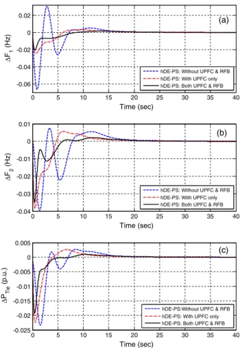
0 5 10 15 20 25 30 35 40 -0.06 -0.04 -0.02 0 0.02 Time (sec) Δ F1 (Hz) (a)

0 5 10 15 20 25 30 35 40 -0.04 -0.03 -0.02 -0.01 0 0.01 Time (sec) Δ F2 (Hz) (b)

0 5 10 15 20 25 30 35 40 -0.025 -0.02 -0.015 -0.01 -0.005 0 0.005 Time (sec) Δ PTie (p.u.) (c)

hDE-PS:Without UPFC & RFB hDE-PS: With UPFC only hDE-PS: Both UPFC & RFB

Figure 12 Dynamic responses of the system for contract violation based scenario (a) frequency deviation of area-1 (b) frequency deviation of area-2 (c) tie-line power deviation.

Table 10 Sensitive analysis under Poolco based transaction.

Parameter variation % Change Settling time in (s) Peak over shoot·103 _ITAE

DF1 DF2 DPTie DF1 DF2 DPTie Nominal 0 19.07 18.09 12.69 0.8 1.7 0.6 0.3858 Changed DPM 19.13 18.15 12.65 0.7 1.7 0.6 0.3868 Loading Condition 25 19.07 18.08 12.69 0.8 1.7 0.6 0.3858 +25 19.08 18.10 12.69 0.8 1.7 0.6 0.3858 TG 25 19.08 18.10 12.69 0.8 1.7 0.6 0.3850 +25 19.06 18.08 12.69 0.8 1.7 0.6 0.3866 TT 25 19.12 18.14 12.69 0.7 1.7 0.6 0.3840 +25 19.02 18.04 12.69 0.8 1.7 0.6 0.3877 TGH 25 19.17 18.18 12.74 0.8 1.7 0.6 0.3699 +25 19.00 18.03 12.66 0.8 1.7 0.6 0.4046 T12 25 19.27 17.69 12.82 0.7 1.9 0.6 0.3895 +25 18.99 18.33 12.54 0.8 1.6 0.5 0.3832 R 25 19.20 17.80 13.00 0.7 1.6 0.7 0.3922 +25 19.09 18.25 12.50 0.8 1.7 0.5 0.3807

(13)

load disturbance of 1% is applied in area-1 and the optimized controller parameters and the corresponding performance index are provided in Table 5. It is clear from Table 5that, the objective function ITAE value is further reduced to

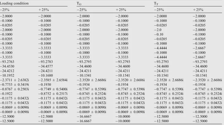
1.0088 with only UPFC controller and smallest ITAE value (ITAE = 0.3858) is obtained with the coordinated application of UPFC and RFB. The improvements in ITAE value for above cases are 40.64% with IPFC only and 77.3% with Table 11 System eigen values under parameter (loading, TGand TT) variation with poolco based transaction.

Loading condition TG TT 25% +25% 25% +25% 25% +25% 2.0000 2.0000 2.0000 2.0000 2.0000 2.0000 0.1000 0.1000 0.1000 0.1000 0.1000 0.1000 0.0205 0.0205 0.0205 0.0205 0.0205 0.0205 2.0000 2.0000 2.0000 2.0000 2.0 2.0000 0.1000 0.1000 0.1000 0.1000 0.10 0.1000 0.0205 0.0205 0.0205 0.0205 0.0205 0.0205 0.1000 0.1000 0.1000 0.1000 0.1000 0.1000 3.3333 3.3333 3.3333 3.3333 4.4444 2.6667 0.1000 0.1000 0.1000 0.1000 0.1000 0.1000 3.3333 3.3333 3.3333 3.3333 4.4444 2.6667 93.2763 93.2783 93.2793 93.2793 93.2793 93.2793 34.4530 34.4577 34.4600 34.4600 34.4600 34.4600 24.4212 24.4211 24.4211 24.4211 24.4211 24.4211 10.1952 10.1680 10.1541 10.1541 10.1541 10.1541

2.3711 ± 2.6382i 2.3585 ± 2.6584i 2.3520 ± 2.6686i 2.3520 ± 2.6686i 2.3520 ± 2.6686i 2.3520 ± 2.6686i

0.7753 ± 0.5419i 0.1930 0.1934 0.1934 0.1934 0.1934

0.8767 ± 0.2503i 0.7749 ± 0.5400i 0.7747 ± 0.5390i 0.7747 ± 0.5390i 0.7747 ± 0.5390i 0.7747 ± 0.5390i

0.1922 0.8752 ± 0.2517i 0.8745 ± 0.2524i 0.8745 ± 0.2524i 0.8745 ± 0.2524i 0.8745 ± 0.2524i

0.1175 ± 0.0432i 0.1175 ± 0.0432i 0.1175 ± 0.0432i 0.1175 ± 0.0432i 0.1175 ± 0.0432i 0.1175 ± 0.0432i

0.0069 ± 0.0090i 0.0069 ± 0.0090i 0.0069 ± 0.0090i 0.0069 ± 0.0090i 0.0069 ± 0.0090i 0.0069 ± 0.0090i

12.5000 12.5000 16.6667 10.0000 12.5000 12.5000

Table 12 System eigen values under parameter (TGH, T12andR) variation with poolco based transaction.

TGH T12 R 25% +25% 25% +25% 25% +25% 2.0000 2.0000 2.0000 2.0000 2.0000 2.0000 0.1000 0.1000 0.1000 0.1000 0.1000 0.1000 0.0274 0.0164 0.0205 0.0205 0.0205 0.0205 2.0000 2.0000 2.0000 2.0000 2.0000 2.0000 0.1000 0.1000 0.1000 0.1000 0.1000 0.1000 0.0274 0.0164 0.0205 0.0205 0.0205 0.0205 0.1000 0.1000 0.1000 0.1000 0.1000 0.1000 3.3333 3.3333 3.3333 3.3333 3.3333 3.3333 0.1000 0.1000 0.1000 0.1000 0.1000 0.1000 3.3333 3.3333 3.3333 3.3333 3.3333 3.3333 93.2793 93.2793 93.2780 93.2807 93.2792 93.2794 34.4600 34.4600 34.4581 34.4619 31.9898 35.7676 24.4211 24.4211 24.4212 24.4211 24.4363 24.4119 10.1541 10.1541 10.3104 9.9941 9.9025 10.2328

2.3520 ± 2.6686i 2.3520 ± 2.6686i 2.3525 ± 2.6184i 2.3547 ± 2.7226i 3.7344 ± 0.3817i 1.6575 ± 3.0849i

0.1934 0.1934 0.7720 ± 0.4520i 0.1950 0.7145 ± 0.5839i 0.8003 ± 0.5127i

0.7747 ± 0.5390i 0.7747 ± 0.5390i 0.8016 ± 0.2530i 0.8106 ± 0.5947i 0.9079 ± 0.2368i 0.8533 ± 0.2570i

0.8745 ± 0.2524i 0.8745 ± 0.2524i 0.1904 0.9134 ± 0.2519i 0.1887 0.1963

0.1175 ± 0.0432i 0.1175 ± 0.0432i 0.1175 ± 0.0432i 0.1175 ± 0.0432i 0.1175 ± 0.0432i 0.1175 ± 0.0432i

0.0069 ± 0.0090i 0.0069 ± 0.0090i 0.0069 ± 0.0090i 0.0069 ± 0.0090i 0.0069 ± 0.0090i 0.0069 ± 0.0090i

12.5000 12.5000 12.5000 12.5000 12.5000 12.5000

(14)

coordinated application of UPFC and RFB compared the sys-tem without UPFC and RFB. The performance indexes in terms of settling time and peak overshoots are accordingly reduced.Fig. 9a–c shows the dynamic performance of the sys-tem with/without UPFC and RFB for the above disturbance. It can be seen from Fig. 9a–c that the system is oscillatory without UPFC and RFB. The dynamic performance is improved with UPFC and signiﬁcant improvement in system performance is obtained with coordinated application of UPFC and RFB.

The performance of proposed hDE-PS optimized MID controller is also evaluated under changed contract participa-tion factor. The following modiﬁed DPM is considered:

DPM¼ 0:4 0:4 0 0 0:4 0:4 0 0 0:2 0:2 0 0 0 0 0 0 0 0 0 0 0 0 0 0 2 6 6 6 6 6 6 6 6 4 3 7 7 7 7 7 7 7 7 5 ð23Þ

The calculated generations under modiﬁed DPM are:

DPg1= 0.004 pu MW, DPg2= 0.004 pu MW, DPg3= 0.002

pu MW and DPg4=DPg5=DPg6= 0 pu MW. A step load

disturbance of 1% is applied in area-1 and the corresponding performance indexes are also provided in Table 5. The dynamic performance of the system for the above changed contract participation factor is shown in Fig. 10a–c. It can be seen fromTable 5andFig. 10a–c that the proposed con-troller is robust and performs satisfactorily with change of contract participation factor.

4.3. Bilateral based transaction

In this scenario, DISCOs have the freedom to contract with any of the GENCOs within or with other areas and it is assumed that a step load disturbance of 0.005 pu MW is demanded by each DISCO in both areas i.e. DPL1¼0:005

pu MW, DPL2¼0:005 pu MW, DPL3¼0:005 pu MW and

DPL4¼0:005 pu MW as result of the total load disturbance

in area-1 is DPD1¼0:01 pu MW and in area-2 is

DPD2¼0:01 pu MW.

From Eq. (3)the deviation in scheduled tie-line power is 0.0015 pu MW. All the GENCOs are participating in the LFC task as per the following DPM.

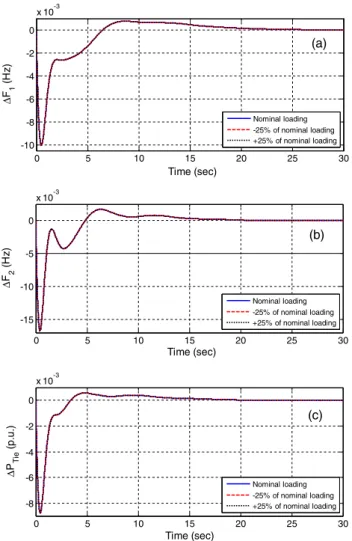
0 5 10 15 20 25 30 -10 -8 -6 -4 -2 0 x 10-3 Δ F1 (H z ) (a) Nominal loading -25% of nominal loading +25% of nominal loading 0 5 10 15 20 25 30 -15 -10 -5 0 x 10-3 Time (sec) Δ F2 (H z ) (b) Nominal loading -25% of nominal loading +25% of nominal loading 0 5 10 15 20 25 30 -8 -6 -4 -2 0 x 10-3 Time (sec) Δ PTi e ( p .u .) (c) Nominal loading -25% of nominal loading +25% of nominal loading Time (sec)

Figure 13 Dynamic responses of the system with variation of loading condition (a) frequency deviation of area-1 (b) frequency deviation of area-2 (c) tie-line power deviation.

0 5 10 15 20 25 30 -10 -8 -6 -4 -2 0 x 10-3 (a) Time (sec) Δ F1 (Hz) Nominal -25% of T G +25% of T_G 0 5 10 15 20 25 30 -15 -10 -5 0 x 10-3 Time (sec) Δ F2 (Hz) (b) Nominal -25% of T_G +25% of T G 0 5 10 15 20 25 30 -8 -6 -4 -2 0 x 10-3 Time (sec) Δ PTie (p.u.) (c) Nominal -25% of T_G +25% of T G

Figure 14 Dynamic responses of the system with variation of TG (a) frequency deviation of area-1 (b) frequency deviation of area-2 (c) tie-line power deviation.

(15)

DPM¼ 0:2 0:1 0:3 0 0:2 0:25 0:1 0:1666 0:1 0:25 0:1 0:1666 0:2 0:1 0:1 0:3666 0:2 0:2 0:2 0:1666 0:1 0:1 0:2 0:1666 2 6 6 6 6 6 6 6 6 4 3 7 7 7 7 7 7 7 7 5 ð24Þ

From Eq. (21) the values of steady-state power generated by the GENCOs can be obtained as: DPg1¼0:003 pu MW,

DPg2¼0:0036 pu MW, DPg3¼0:0031 pu MW, DPg4¼

0:0038 pu MW, DPg5¼0:0038 pu MW and DPg6¼0:0028

pu MW.

The tuned MID controller parameters for Bilateral based transaction are given in Table 6. The various performance indexes (ITAE, settling time and peak overshoot) under bilat-eral based transaction case are given inTable 7. It is clear from

Table 7 that minimum ITAE value is obtained with coordi-nated application of UPFC and RFB (ITAE = 0.5033) com-pared to only UPFC (ITAE = 1.0331) and without UPFC and RFB optimized MID controller (ITAE = 2.0231). The improvements in ITAE value for above case are 48.93% with UPFC only and 75.12% with coordinated application of UPFC and RFB. Consequently, better system performance

in terms of minimum settling times in frequency and tie-line power deviations is achieved with proposed UPFC and RFB optimized MID controller compared to others as shown in

Table 7. Hence it can be concluded that in this case also, the coordination of IPFC and RFB works satisfactorily. The sys-tem dynamic responses are shown in Fig. 11a–c. From

Fig. 11a–c, it shows that coordinated application of UPFC and RFB signiﬁcantly improves the dynamic performance of the system. Improved results in settling times and peak over-shoots of DF1, DF2 and DPTie are obtained with proposed

hDE-PS optimized MID controller with coordinated applica-tion of UPFC and RFB compared to others.

4.4. Contract violation

It may happen that DISCOs may violate a contract by demanding more than that specified in the contract. This excess power is not contracted out to any GENCO. This un-contracted power must be supplied by the GENCOs in the same area as that of the DISCOs. It must be reflected as a local load of the area but not as the contract demand. Considering scenario 2 (bilateral based transaction) again with a modifica-tion that 0.01 (pu MW) of excess power demanded by

0 5 10 15 20 25 30 -10 -8 -6 -4 -2 0 x 10-3 Time (sec) Δ F1 (Hz) (a) Nominal -25% of T T +25% of T_T 0 5 10 15 20 25 30 -15 -10 -5 0 x 10-3 Time (sec) Δ F2 (Hz) (b) Nominal -25% of T T +25% of T_T 0 5 10 15 20 25 30 -8 -6 -4 -2 0 x 10-3 Time (sec) Δ PTie (P.u.) (c) Nominal -25% of T_T +25% of T T

Figure 15 Dynamic responses of the system with variation of TT (a) frequency deviation of area-1 (b) frequency deviation of area-2 (c) tie-line power deviation.

0 5 10 15 20 25 30 -10 -8 -6 -4 -2 0 x 10-3 Time (sec) Δ F1 (Hz) (a) Nominal -25% of T GH +25% of T_GH 0 5 10 15 20 25 30 -15 -10 -5 0 x 10-3 Time (sec) Δ F2 (Hz) (b) Nominal -25% of T_GH +25% of T_GH 0 5 10 15 20 25 30 -8 -6 -4 -2 0 x 10-3 Time (sec) Δ PTie (p.u.) (c) Nominal -25% of T GH +25% of T GH

Figure 16 Dynamic responses of the system with variation of TGH(a) frequency deviation of area-1 (b) frequency deviation of area-2 (c) tie-line power deviation.

(16)

DISCO1. Now DPD1 becomes, DPD1¼DPL1þDPL2þ

DPuc1¼0:02 (pu MW) while DPD2 remains unchanged. As

there is contract violation, the values ofDPg1,DPg2 andDPg3

are to be changed. The change in violation of powers calcu-lated as follows:

DPg1;violation¼DPg1þapf11DPviolation¼0:009 p:u MW ð25Þ

DPg2;violation¼DPg2þapf12DPviolation¼0:0066 pu MW ð26Þ

DPg3;violation¼DPg3þapf13DPuc1¼0:0041 pu MW ð27Þ

The values ofDPg4,DPg5andDPg6are same as in scenario 2

(bilateral based transaction).

Table 8gives the tuned MID controller parameters for con-tract violation based transaction. The various performance indexes in terms of ITAE, settling time and peak overshoot for the above case are given inTable 9. It can be seen from

Table 9that superior results are obtained with coordinated application of UPFC and RFB compared to others. The improvements in ITAE value for contract violation based transaction are 36.91% with UPFC only and 64.78% with coordinated application of UPFC and RFB. The frequency deviations and tie-line power are shown inFig. 12a–c. It is evi-dent from Fig. 12a–c that with coordinated application of UPFC and RFB the oscillations are quickly damped out.

4.5. Sensitivity analysis

Robustness is the ability of a system to perform effectively while its variables are changed within a certain tolerable range[21,26,28]. In this section robustness of the power sys-tem is checked by varying the loading conditions and syssys-tem parameters from their nominal values (given in Appendix A) in the range of +25% to 25% without changing the opti-mum values of proposed MID controller gains. The change in operating load condition affects the power system param-eters KPS andTPS. The power system parameters are

calcu-lated for different loading conditions as given in Appendix A. The system with UPFC and RFB under poolco based scenario is considered in all the cases due to their superior performance. The various performance indexes (ITAE values, settling times and peak overshoot) under normal and param-eter variation cases for the system are given in Table 10. It can be observed from Table 10that the ITAE, settling time and peak overshoot values are varying within acceptable ranges and are nearby equal to the respective values obtained with nominal system parameter. The system modes under these cases are shown in Tables 11 and 12. It is also evident fromTables 11 and 12that the eigen values lie in the left half

0 5 10 15 20 25 30 -10 -8 -6 -4 -2 0 x 10-3 Time (sec) Δ F1 (Hz) (a) Nominal -25% of T₁₂ +25% of T₁₂ 0 5 10 15 20 25 30 -15 -10 -5 0 x 10-3 Time (sec) Δ F2 (Hz) (b) Nominal -25% of T 12 +25% of T 12 0 5 10 15 20 25 30 -8 -6 -4 -2 0 x 10-3 Time (sec) Δ PTie (p.u.) (c) Nominal -25% of T₁₂ +25% of T₁₂

Figure 17 Dynamic responses of the system with variation of T12 (a) frequency deviation of area-1 (b) frequency deviation of area-2 (c) tie-line power deviation.

0 5 10 15 20 25 30 -10 -8 -6 -4 -2 0 x 10-3 Time (sec) Δ F1 (Hz) (a) Nominal -25% of R +25% of R 0 5 10 15 20 25 30 -15 -10 -5 0 x 10-3 Time (sec) Δ F2 (Hz) (b) Nominal -25% of R +25% of R 0 5 10 15 20 25 30 -8 -6 -4 -2 0 x 10-3 Time (sec) Δ PTie (p.u.) (c) Nominal -25% of R +25% of R

Figure 18 Dynamic responses of the system with variation ofR

(a) frequency deviation of area-1 (b) frequency deviation of area-2 (c) tie-line power deviation.

(17)

of s-plane for all the cases thus maintain the stability

[26,28,29,30]. Hence, it can be concluded that the proposed MID controller in deregulation environment is very much robust and performs satisfactorily when system parameters changes in the range of ±25%.

The dynamic performances of the system under variation of parameters are shown inFigs. 13–18. It can be observed from

Figs. 13–18that the effect of the variation of operating loading conditions on the system responses is negligible. Hence it can be concluded that, the proposed control strategy provides a robust control under wide changes in the loading condition and system parameters. Further, to investigate the superiority of the proposed method, a random step load changes are applied in area-1 i.e.under poolco based scenario. Figs. 19a and 19b show the random load pattern of power system. The step loads are random both in magnitude and duration. The frequency response for random load disturbance in area-1 is shown inFigs. 19c and 19d. FromFigs. 19c and 19d, it is evident that proposed method shows better transient

response when the system is incorporated with UPFC and RFB than other.

It is worth mentioning that, the controllers are designed ofﬂine during planning stage and then put into action for online control of power system. So before the controllers are put into operation, the parameters are determined and they remain ﬁxed. Therefore, the complexity of using pro-posed hybrid method to determine the controller parameters will not increase the computational burdens during online applications.

5. Conclusion

In this paper, an attempt has been made for the first time to apply a hybrid Differential Evolution (DE) and Pattern Search (PS) optimized Modified Integral Derivative (MID) controller for load frequency control of area multi-source power system in deregulated environment. The Boiler dynamics, Generation Rate Constraint (GRC) and Governor Dead Band (GDB) have been considered to have a more real-istic power system. The system has been investigated all possi-ble of power transactions that take place under deregulated environment. The proposed hybrid technique takes advantage of global exploration capabilities of DE and local exploitation capability of PS. The advantage of proposed hDE-PS tech-nique over DE and Genetic Algorithm (GA) has also been demonstrated. It is observed that better dynamic performance is obtained with proposed hDE-PS optimized MID controller compared to I and ID controller. Unified Power Flow Controller (UPFC) is added in the tie-line for improving the system performance. Additionally, Redox Flow Batteries (RFBs) are included in area-1 along with UPFC in order to improve the system performance. It is observed that in all the cases (poolco based, bilateral based and contract violation based) the deviation of frequency becomes zero in the steady state with coordinated application of UPFC and RFB which assures the AGC requirements. Additionally, sensitivity analy-sis is carried out to show the robustness of the MID controller under poolco based scenario. From simulation results, it is observed that the parameters of the proposed hDE-PS opti-mized MID controllers are need not be reset even if the system is subjected to wide variation in loading condition and system parameters. Finally, the simulation results are demonstrated that the proposed approach provides desirable performance against random step load disturbance.

0 20 40 60 80 100 120 140 160 180 200 -0.05 0 0.05 0.1 Time (sec) Δ PD (p.u.) (a)

Figure 19a Random step load pattern varied from0.05 pu to 0.1 pu. 0 20 40 60 80 100 120 140 160 180 200 -5 -2.5 0 2.5 5x 10 -3 Time (sec) Δ PD (p.u.) (b)

Figure 19b Random step load pattern varied from0.005 pu to 0.005pu. 0 20 40 60 80 100 120 140 160 180 200 -0.4 -0.2 0 0.2 Time (sec) Δ F1 (Hz) (c)

hDE-PS:Without UPFC & RFB hDE-PS:With UPFC only hDE-PS:Both UPFC & RFB

Figure 19c Frequency deviation in area-1 under poolco based scenario for random load pattern varied from0.05 to 0.1 pu.

0 20 40 60 80 100 120 140 160 180 200 -0.015 -0.01 -0.005 0 0.005 0.01 0.015 Time (sec) Δ F1 (Hz) (d)

hDE-PS:Without UPFC & RFB hDE-PS:With UPFC only hDE-PS:Both UPFC & RFB

Figure 19d Frequency deviation in area-1 under poolco based scenario for random load pattern varied from0.005 to 0.005pu.

(18)

Appendix A

Nominal parameters of the system investigated are as follows: A.1. Two area multisource thermal hydro wind diesel power system [19] F¼60 Hz; B1¼B2¼0:425 p.u.MW/Hz; R1¼R2¼R3¼ R4¼R5¼R6¼2:4 Hz/p.u.; TG1¼TG2¼0:08 s; TT1¼ TT2¼0:3 s; Kr1¼Kr2¼0:333, Tr1¼Tr2¼10 s, TGH1¼ TGH2¼48:7 s; TRS1¼TRS2¼0:513; TRH1¼TRH2¼10; TW1¼1; Kdiesel¼16:5; KP1¼1:25; KP2¼1:4; TP1¼6; TP2¼0:041; K1¼0:85; K2¼0:095; K3¼0:92; KIB¼0:03; TIB¼26; TRB¼6:9; CB¼200; TD¼0; TF¼10; KPS1¼ KPS2¼120 Hz/p.u.MW; TPS1¼TPS2¼20 s; T12¼0:0866 pu;a12¼ 1.

A.2. Data for UPFC & RFB

TUPFC¼0:01 s;KRFB¼0:67;TRFB¼0 s.

References

[1]Elgerd OI. Electric energy systems theory – an introduction. New Delhi: Tata McGraw Hill; 2000.

[2]Bevrani H. Robust power system frequency control. Springer; 2009.

[3]Bervani H, Hiyama T. Intelligent automatic generation control. CRC Press; 2011.

[4]Donde V, Pai MA, Hiskens IA. Simulation and optimization in an AGC system after deregulation. IEEE Trans Power Syst 2011;16:481–9.

[5]Christie RD, Bose A. Load frequency control issues in power system operation after deregulation. IEEE Trans Power Syst 1996;11:1191–2000.

[6]Parmar KPS, Majhi S, Kothari DP. LFC of an interconnected power system with multi-source power generation in deregulated power environment. Int J Elect Power Energy Syst 2014;57: 277–86.

[7]Debbarma S, Saikia LC, Sinha N. AGC of a multi-area thermal system under deregulated environment using a non-integer con-troller. Electric Power Syst Res 2013;95:175–83.

[8]Demiroren A, Zeynelgil HL. GA application to optimization of AGC in three-area power system after deregulation. Int J Elect Power Energy Syst 2007;29:230–40.

[9]Bhatt P, Roy R, Ghoshal SP. Optimized multi area AGC simulation in restructured power systems. Int J Elect Power Energy Syst 2010;32:311–32.

[10]Saikia LC, Nanda J, Sinha N. Performance comparison of several classical controllers in AGC for multi-area interconnected thermal system. Int J Elect Power Energy Syst 2011;33:394–401. [11]Tan W, Zhang H, Yu M. Decentralized load frequency control in

deregulated environments. Int J Elect Power Energy Syst 2012;41:16–26.

[12]Liu F, Song YH, Ma J, Mei S, Lu Q. Optimal load–frequency control in restructured power systems. IEE Proc Gen Trans Distribution 2003;150(1):87–95.

[13]Das D, Aditya SK, Kothari DP. Dynamics of diesel and wind turbine generators on an isolated power system. Int J Elect Power Energy Syst 1999;21:183–9.

[14]Hingorani NG, Gyugyi L. Understanding FACTS: concepts and technology of ﬂexible AC transmission system. IEEE Press; 2000.

[15] Sasaki T, Kadoya T, Kazuhiro E. Study on load frequency control using redox ﬂow batteries. IEEE Trans Power Syst 2004;19(1):660–7.

[16] Enomoto K, Sasaki T, Shigematsu T, Deguchi H. Evaluation study about redox ﬂow battery response and its modelling. IEEJ Trans Power Eng 2002;122(4):554–60.

[17] Chidambaram IA, Paramasivam B. Optimized load–frequency simulation in restructured power system with redox ﬂow batteries and interline power ﬂow controller. Int J Elect Power Energy Syst 2013;50:9–24.

[18] Dolan ED, Lewis RM, Torczon V. On the local convergence of pattern search. SIAM J Optimiz 2003;14(2):567–83.

[19] Mohanty B, Panda S, Hota PK. Differential evolution algorithm based automatic generation control for interconnected power systems with non-linearity. Alexandria Eng J 2014;53(3): 537–52.

[20] Khuntia SR, Panda S. Simulation study for automatic generation control of a multi-area power system by ANFIS approach. Appl Soft Comput 2012;12(1):333–41.

[21] Sahu RK, Panda S, Padhan S. Optimal gravitational search algorithm for automatic generation control of interconnected power systems. Ain Shams Eng J 2014;5(3):721–33.

[22] Panda S. Robust coordinated design of multiple and multi-type damping controller using differential evolution algorithm. Int J Elect Power Energy Syst 2011;33:1018–30.

[23] Kazemi A, Shadmesgaran MR. Extended supplementary Controller of UPFC to improve damping inter-area oscillations considering inertia coefﬁcient. Int J Energy 2008;2(1):25–36. [24] Parmar KPS. Load frequency control of multi-source power

system with redox ﬂow batteries: an analysis. Int J Computer Appl 2014;88(8):46–52.

[25] Stron R, Price K. Differential evolution – a simple and efﬁcient adaptive scheme for global optimization over continuous spaces. J Global Optimiz 1995;11:341–59.

[26] Sahu RK, Panda S, Rout UK. DE optimized parallel 2-DOF PID controller for load frequency control of power system with governor dead-band nonlinearity. Int J Elect Power Energy Syst 2013;49(1):19–33.

[27] Othman AK, Ahmed AN, AlSharidah ME, AlMekhaizim HA. A hybrid real coded genetic algorithm – pattern search approach for selective harmonic elimination of PWM AC/AC voltage con-troller. Int J Elect Power Energy Syst 2013;44:123–33.

[28] Rout UK, Sahu RK, Panda S. Design and analysis of differential evolution algorithm based automatic generation control for interconnected power system. Ain Shams Eng J 2013;4(3): 409–21.

[29] Debbarma S, Saikia LC, Sinha N. Automatic generation control using two degree of freedom fractional order PID controller. Int J Elect Power Energy Syst 2014;58:120–9.

[30] Ali ES, Abd-Elazim SM. Bacteria foraging optimization algo-rithm based load frequency controller for interconnected power system. Int J Elect Power Energy Syst 2011;33(3):633–8.

Rabindra Kumar Sahu received the Ph.D. degree from the Indian Institute of Technology (IIT) Madras, Chennai, India. He is currently working as Associate Professor and Head of the Department, Electrical Engineering & EEE, Veer Surendrai Sai University of Technology (VSSUT), Burla, Sambalpur, Odisha, India. His research interests include application of soft computing techniques to power system engineering, Flexible AC Transmission Systems (FACTS). Dr. Sahu is a life member of ISTE.

(19)

G.T. Chandra Sekharreceived B.Tech degree in EEE from St. Theressa institute of Engineering & Technology, Vizianagaram afﬁliated to JNTU, Hyderabad, Andhra Pradesh in 2008. M.Tech Degree in EEE from St. Theressa institute of Engineering & Technology, Vizianagaram afﬁliated to JNTU, Kakinada, Andhra Pradesh in 2011. He is currently working toward the Ph.D. degree at the Department of Electrical Engineering, VSSUT, Burla, Odisha, India. His research interests include soft computing application in power system Engineering. Mr. Chandra Sekhar is a life member of ISTE.

Sidhartha Pandareceived Ph.D. degree from Indian Institute of Technology (IIT), Roorkee, India, M.E. degree from Veer Surendrai Sai University of Technology (VSSUT). Presently, he is working as a Professor in the Department of Electrical Engineering, Veer Surendrai Sai University of Technology (VSSUT), Burla, Sambalpur, Odisha, India. His areas of research include Flexible AC Transmission Systems (FACTS), Power System Stability, Soft computing, Model Order Reduction, Distributed Generation and Wind Energy. Dr. Panda is a Fellow of Institution of Engineers (India).