Approach of economic‐emission load dispatch
using Ant Lion Optimizer
Jorge de Almeida Brito Júnior
1, Manoel Henrique Reis Nascimento
2, Carlos
Alberto Oliveira de Freitas
3, Jandecy Cabral Leite
4, Tirso Lorenzo Reyes
Carvajal
51Research department, Institute of Technology and Education Galileo of Amazon - ITEGAM, Manaus, AM, Brazil
Email: [email protected] m
2Research department, Institute of Technology and Education Galileo of Amazon - ITEGAM, Manaus, AM, Brazil
Email: [email protected]
3Research department, Institute of Technology and Education Galileo of Amazon - ITEGAM, Manaus, AM, Brazil
Email: [email protected]
4Research department, Institute of Technology and Education Galileo of Amazon - ITEGAM, Manaus, AM, Brazil
Email: [email protected]
5Research department, Institute of Technology and Education Galileo of Amazon - ITEGAM, Manaus, AM, Brazil
Email: [email protected]
Abstract— To solve the problem of the economic emission load dispatch (EELD) is necessary minimize the total cost of fuel consumption and carbon emission. In this study is applied the ant lion optimizer (ALO) to this problem. The cost function and emission function with their respective restrictions are being using. To present the results this proposal is applied in IEEE 30 bus system that consists of six thermal units. The results for this case study with the application of ant lion with all generators on with demand being met, the total fuel cost is 48915.36652 ($/h). The results this method can be compared with another metaheuristic algorithms and helps the plant operators in the decision mak ing of preventive maintenance.
Keywords—Ant lion Optimizer, EELD, Power Plants.
I. INTRODUCTION
The Thermal Power Plant (TPP) operation is dependent upon incineration of fossil fuel which generates sulfur dioxide (SO2), carbon dioxide (CO2) and nitrogen oxides
(NOx) which create atmospheric pollution. Reduce the
emission level and total cost of generation and at the same time accomplishing the demand for electricity from the power plant is is the goal of economic emission load dispatch (EELD). To solve the EELD problem is necessary minimize the total cost of fuel consumption and carbon emissions (De, Das, Mandal, & Mandal, 2018; Moraes, Bezerra, Moya Rodríguez, Nascimento, & Leite, 2018). The problem is formulated as a multiobjective economic emission load dispatch (EELD) problem in which both the objectives (emission and economy) have
to be minimized (Chopra, Kumar, & Mehta, 2016). This is a complex problem to solve because of its large size, a nonlinear objective function and a wide number of restrictions (Bhattacharya & Chattopadhyay, 2010). Various evolutionary, heuristic and meta-heuristics optimization algorithms have been developed such as: Grey Wolf Optimization (GWO) (Chopra et al., 2016; Hong, MH, & Mohd Rusllim, 2014), non-dominated sorting genetic algorithm (NSGA-II) (Basu, 2008; Moraes et al., 2018), hybrid genetic algorithm (Thenmozhi & Mary, 2004), Tabu Search Algorithm (Li, Yang, Tseng, Wang, & Lim, 2018), Simulated annealing (Júnior, Nunes, Nascimento, Rodríguez, & Leite, 2017; Ziane, Benhamida, & Graa, 2017), Neural Networks (Deng, He, & Zeng, 2017), Harmony Search Algorithm (El Ela, El-Sehiemy, Shaheen, & Shalaby, 2017), particle swarm optimization (De et al., 2018), Differential Evolution (Jebaraj, Venkatesan, Soubache, & Rajan, 2017), Ant Colony Optimization (Zhou et al., 2017), Biogeography-Based Optimization (Ma, Yang, You, & Fei, 2017), genetic algorithm controlled by fuzzy logic (Song, Wang, Wang, & Johns, 1997).
This research use the emission function and economic function in the multiobjective optimization ALO, with restrictions.
II. MATERIAL AND METHODS
To solve a problem of EELD, two important objectives in an electrical power system must be considered; they are: environmental, and economy impacts (Basu, 2014).
The fuel cost is considered as an essential criterion for economics analysis in ELD. The most simplified cost function of each generator can be assumed to be approximated by a quadratic function of generator power output Pi (Ghosh, Chakraborty, Bhowmik, &
Bhattacharya, 2017; Jebaraj et al., 2017):
𝐹1(𝑃𝑖) = ∑(𝑎𝑖+ 𝑏𝑖𝑃𝑖+ 𝑐𝑖𝑃𝑖2) $/ℎ
𝑁
𝑖 =1
(1)
where ai, bi and ci are the fuel cost coefficients of the ith
unit generating, N the number of generators and Pi the
active power of each generator. Fig. 1 illustrates the fuel cost curve without valve-point effects and emissions.
Fig.1: Fuel cost and emission function of the thermal generator.
Source: (Gitizadeh & Ghavidel, 2014)
2.2 Economic Emission Dispatch
Emissions can be represented by a function, that links emissions with power generated by each unit. The emission function in kg/h, which normally represents the emission of SO2 and NOx, is a function of the power output of the generator, and it can be expressed as follows (Swain, Sarkar, Meher, & Chanda, 2017):
𝐹2(𝑃𝑖) = ∑(𝑑𝑖+ 𝑒𝑖𝑃𝑖+ 𝑓𝑖𝑃𝑖2) 𝑘𝑔/ℎ
𝑁
𝑖 =1
(2)
Where di, ei and fi are the emission coefficients of the ith
unit generating, N the number of generators and Pi the
active power of each generator, from the TPP.
2.3 Economical load dispatch constrains
2.3.1 Equality power balance constraint
The real power of each generator is limited by the lower and upper limits. The following equation is the equality restriction of power balance (Rizk-Allah, El-Sehiemy, & Wang, 2018).
∑ 𝑃𝑖− 𝑃𝐷 − 𝑃𝐿
𝑛
𝑖 =1
(2)
where Pi is the output power of each i generator, PD is the
load demand and PL are transmission losses, in other
words, the total power generation has to meet the total demand PD and the actual power losses in transmission lines PL (Dewangan, Jain, & Huddar, 2015).
∑ 𝑃𝑖 = 𝑃𝐷 − 𝑃𝐿
𝑛
𝑖=1
(3)
The calculation of power losses PL involves the solution of the load flow problem, which has equality constraints in the active and reactive power on each bar as follows (Nwulu & Xia, 2015):
𝑃𝐿= ∑ 𝐵
𝑖𝑃𝑖2 𝑛
𝑖 =1
(4)
A simplification is applied to model the transmission losses, setting them as a function of the generator output
through Kron’s loss coefficient derivatives of the Kron
formula for losses (Huang et al., 2018).
𝑃𝐿= ∑ ∑ 𝑃 𝑖𝐵𝑖𝑗𝑃𝑗+ 𝑛 𝑗=1 ∑ 𝐵0𝑖𝑃𝑖+ 𝑛 𝑖 =1 𝐵00 (5) 𝑛 𝑖=1
where Bij, B0i and B00 are the energy loss coefficients in
the transmission network and n is the number of generators. A reasonable accuracy can be obtained when the actual operating conditions are close to the base case, where the B coefficients were obtained (Gitizadeh & Ghavidel, 2014).
2.3.2 Production Capacity Constraint
The power capacity total generated from each generator is restricted by the lower limit and by the upper limit, so the constrain is (De et al., 2018):
𝑃𝑚𝑖𝑛 .𝑖≤ 𝑃𝑖 ≤ 𝑃𝑚𝑎𝑥 .𝑖 (6)
where Pi is the output power of the i generator, Pmin.i, is
the minimal power of the i generator and Pmax.i, the
maximal power of the i generator. 2.3.3 Fuel Delivery Constraint
At each time interval, the amount of fuel supplied to all units must be less than or equal to the fuel supplied by the seller, i.e. the fuel delivered to each unit in each interval should be within its lower limit Fmin,i and its upper limit
Fmax,i so that (Qu et al., 2018):
𝐹𝑚𝑖𝑛 .𝑖 ≤ 𝐹𝑖𝑚 ≤ 𝐹𝑚𝑎𝑥 .𝑖, 𝑖 ∈ 𝑁 , 𝑚 ∈ 𝑀, (7)
where Fi,m is the fuel supplied to the engine i at the interval
m, Fi,min is the minimum amount of fuel supplied to i
generator and Fmax,i is the maximum amount of fuel
supplied to i generator. 2.3.4 Optimization problem
The multi-objective optimization problem is defined as follow:
𝑀𝑖𝑛𝑖𝑚𝑖𝑧𝑒 (𝑃) = [𝐹1(𝑃), 𝐹2(𝑃) ] (8)
where F1(P), F2(P) are the objective functions to be
minimized over the set of permissible decision vector P. 2.3.5 Incremental fuel cost method
The incremental fuel cost can be obtained from the following equation (Tiwari, Dave, & Dwivedi, 2017):
𝐼𝐶𝑖= (2. 𝑎𝑖. 𝑃𝑔 𝑖 + 𝑏𝑖) $/𝑀𝑊ℎ (9)
where ICi is the incremental fuel cost ai are the values of
the different points of the actual curve of the incremental cost and bi are the values of the points on the
approximated curve (linear) of incremental cost. Pgi is the
total power generation. The curve of incremental fuel cost is show in the following Figure. 2:
Fig.2: Incremental Cost Curve of Power Generator. Source:(Nascimento, Nunes, Rodríguez, Leite, & Junior,
2016)
2.4 Ant lion optimization
The Ant Lion Optimizer (ALO) is a algorithm ins pired by nature (Mirjalili, 2015). The ALO algorithm mimics interaction between antlions and ants in the trap. To model such interactions, ants are required to move over the search space, and antlions are allowed to hunt them and become fitter using traps. Since ants move stochastically in nature when searching for food, a random walk is
chosen for modelling ants’ movement as follows [28]:
where cumsum calculates the cumulative sum, n is the maximum number of iteration, t shows the step of random walk (iteration in this study), and r(t) is a stochastic function defined as follows (Trivedi, Jangir, & Parmar, 2016):
𝑟(𝑡) = {1 𝑖𝑓 𝑟𝑎𝑛𝑑 > 0.5
0 𝑖𝑓 𝑜𝑡ℎ𝑒𝑟𝑤𝑖𝑠𝑒 (11)
where t shows the step of random walk (iteration in this study) and rand is a random number generated with uniform distribution in the interval of [0, 1].
To keep the random walk in the boundaries of the search space and prevent the ants from overshooting, the random walks should be normalized using the following equatio n (Yao & Wang, 2017):
𝑋𝑖𝑡 =
(𝑋𝑖𝑡−𝑎𝑖)×(𝑑𝑖𝑡−𝑐𝑖𝑡) (𝑏𝑖−𝑎𝑖) + 𝑐𝑖
𝑡 (12)
where 𝑐𝑖𝑡 is the minimum of i-th variable at t-th iteration, 𝑑𝑖𝑡 indicates the maximum of i-th variable at t-th iteration, 𝑎𝑖 is the minimum of random walk of i-th variable, and 𝑏𝑖
is the maximum of random walk in i-th variable.
To simulate the trapping of ants the mathematical
expression of the trapping of the ants to the ant lion’s pits
is given by following equations (Trivedi et al., 2016):
𝑐𝑚𝑡 = 𝐴𝑛𝑡 − 𝑙𝑖𝑜𝑛𝑛𝑡 − 𝑐𝑡 (13) 𝑑𝑚𝑡 = 𝐴𝑛𝑡 − 𝑙𝑖𝑜𝑛𝑛𝑡 − 𝑑𝑡 (14)
To construction of trap, the fittest ant lion is selected using the roulette wheel method.
To simulate the sliding ants towards ant lions, the boundaries of random walks should be reduced adaptively as follows (Mirjalili, 2015): 𝑐𝑡=𝑐 𝑡 𝐼 (15) 𝑑𝑡=𝑑 𝑡 𝐼 (16) where 𝐼 = 10𝑤 𝑡
𝑠, t is current iteration, S is the maximum
number of iterations and w is a constant whose value is given by (Raju, Saikia, & Sinha, 2016):
𝑤 = { 2 𝑖𝑓 𝑡 > 0.1𝑆 3 𝑖𝑓 𝑡 > 0.5𝑆 4 𝑖𝑓 𝑡 > 0.75𝑆 5 𝑖𝑓 𝑡 > 0.9𝑆 6 𝑖𝑓 𝑡 > 0.95𝑆 (17)
To catching the ants by ant lion and re-building the pit can be mathematically described as [28]:
𝐴𝑛𝑡𝑙𝑖𝑜𝑛𝑗𝑡= 𝐴𝑛𝑡𝑖𝑡, 𝑖𝑓 𝑓(𝐴𝑛𝑡𝑖𝑡) > 𝑓(𝐴𝑛𝑡𝑙𝑖𝑜𝑛𝑗𝑡) (18)
where 𝐴𝑛𝑡𝑙𝑖𝑜𝑛𝑗𝑡 indicates the position of selected jth ant
lion at tth iteration and 𝐴𝑛𝑡𝑖𝑡 shows the position of ith ant
at tth iteration. t shows the current iteration.
Finally the last operator in ALO, that is elitism, calculated using roulette wheel as follows equation (Trivedi et al., 2016):
𝐴𝑛𝑡𝑖𝑡=
𝑅𝐴𝑡 + 𝑅𝐸𝑡
2 (19)
where, 𝑅𝐴𝑡 = the random walk nearby the ant lion chose by
means of the roulette wheel at tth iteration, 𝑅
𝐸𝑡 = the
random walk nearby the elite at tth iteration, 𝐴𝑛𝑡 𝑖𝑡 = the
location of ith ant at tth iteration.
2.5 ALO applied to EELD
Initialize random walks on ants using Eq (10) and save generation scheduling of generating units as ant position using Eq (20) described below:
where 𝑀𝐴𝑛𝑡 is the matrix for saving the position of each
ant, 𝐴𝑛𝑡𝑖,𝑗 shows the value of the jth variable (dimension)
of ith ant, n is the number of ants, and d is the number of variables.
For evaluating each ant (i.e., generating units), the following objective functions described in Eq. (1) and Eq (2) are utilized during optimization and following matrix stores the fitness value of all ants:
where 𝑀𝑂𝐴 is the matrix for saving the fitness of each ant, 𝐴𝑛𝑡𝑖 ,𝑗 shows the value of jth dimension of ith ant, n is the
number of ants, and f is the objective function.
Save the optimal cost and generation scheduling using Eqs. (22) and (23) described below:
where 𝑀𝑂𝐴𝐿 is the matrix for saving the fitness of each ant
lion, 𝐴𝐿𝑖,𝑗 shows the jth dimension’s value of ith ant lion,
n is the number of ant lions, and f is the objective function. This solution comprises the number of generations of the system that will be optimized, which results in minimization of cost and emissions described in Eq (8) by fulfilling all constraints described in Eq (3), Eq (6) and Eq (7).
Equation (8) are applied in the performance evaluation of the EELD until the optimum cost and emission is achieved. For inequality constraints, similar to any other techniques, when the solutions obtained for any iteration are out of boundaries, ALO chooses the boundaries values, while for equality constraint, when it is violated, the penalty factor of 1000 is implemented and embedded in the cost function as per Eq. (8). The algorithm will continue until the maximum iteration is met, and the optimum results are obtained.
III. SIMULATION TESTS AND RESUTS
The power plant selected for the case study consists of six generating units with a load demand of 900 MW where generation limits, fuel cost and emission coefficients for case study is take from Ref (Lee & Darwish, 2008; Manteaw & Odero, 2012).
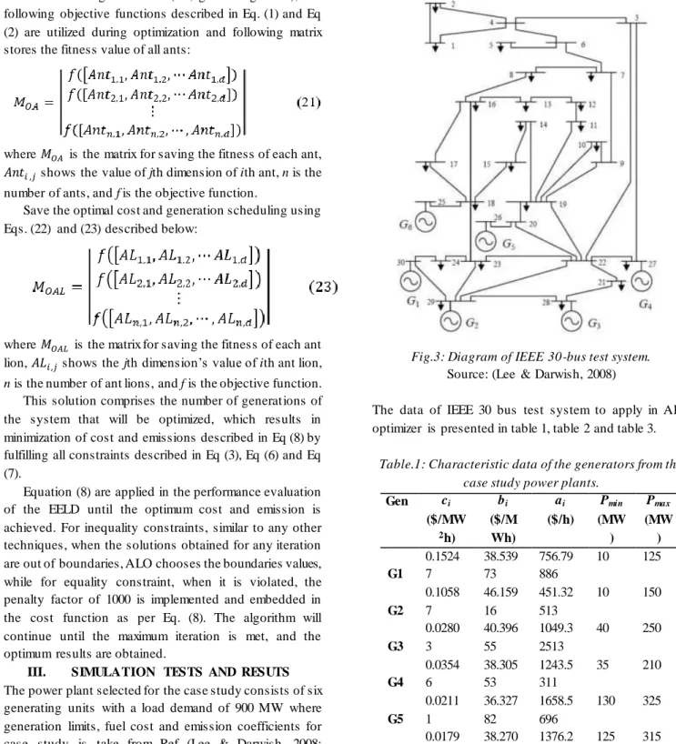
The EELD problem simulated with the ALO algorithm, the systems of standard IEEE 30 bus systems have been taken into consideration (figure 3).
Fig.3: Diagram of IEEE 30-bus test system. Source: (Lee & Darwish, 2008)
The data of IEEE 30 bus test system to apply in ALO optimizer is presented in table 1, table 2 and table 3.
Table.1: Characteristic data of the generators from the case study power plants.
Gen ci ($/MW 2h) bi ($/M Wh) ai ($/h) Pmin (MW ) Pmax (MW ) G1 0.1524 7 38.539 73 756.79 886 10 125 G2 0.1058 7 46.159 16 451.32 513 10 150 G3 0.0280 3 40.396 55 1049.3 2513 40 250 G4 0.0354 6 38.305 53 1243.5 311 35 210 G5 0.0211 1 36.327 82 1658.5 696 130 325 G6 0.0179 9 38.270 41 1376.2 7041 125 315 Source: (Manteaw & Odero, 2012)
Table.2: Coefficients of emission of the 6 generating unit.
Unit di ei fi
G1 0.00419 0.32767 13.85932
G3 0.00683 -0.54551 40.2669 G4 0.00683 -0.54551 40.2669 G5 0.00461 -0.51116 42.89553 G6 0.00461 -0.51116 42.89553
Source: (Manteaw & Odero, 2012) Table.3: Loss coefficients (x10-6).
2022 -286 -534 -565 -454 -103 -286 3243 16 -307 -422 -147 -535 16 2085 831 23 -270 -565 -307 831 1129 113 -295 -454 -422 23 113 460 -153 -103 -147 -270 -295 -153 898
Source: (Manteaw & Odero, 2012)
The results after running the simulation of the proposed ALO algorithm, are displayed in Tables 4.The simulation of the proposed ALO algorithm is tested in MATLAB R2016 to meet the demand of 900MW.
Table.4: Coefficients of emission of the 6 generating unit. Ge ner ato r Power of each generator in Mw Emission of each engine in Kg/h Cost of each engine in $/h G1 125 8238.41182 7956.60886 G2 92.7026704 3382.26922 5640.22656 G3 86.4365762 4403.87432 4750.48463 G4 151.819543 23857.7694 7876.38287 G5 240.571054 64104.5546 11619.7208 G6 229.179195 55417.1514 11071.9428 Tot al 925.709039 159404.0308 48915.36652 Source: Authors
The graphics with pareto front of costs versus emissions and the using all generators is presented in fig. 4.
Fig.4: Pareto front of cost vs emission.
Source: Authors.
The graphics with power, emission and cost are presented in figure 5, 6 and 7 respectively.
Fig.5: Power generated in each generator. Source: Authors.
Fig.6: Emission in each generator. Source: Authors.
Fig.7: Cost of each generator. Source: Authors.
IV. CONCLUSION
The ant lion optimizer is successfully applied to a 30 bus test system, to solve the EELD problem, so now it is possible to use these results to compare with other techniques that apply to this same IEEE bus test system system. This application can also help workers to operate more efficiently the generators in a power plant.
ACKNOWLEDGEMENTS
To the Institute of Technology and Education “Galileo”
from Amazonia (ITEGAM), The Federal University of Para (UFPA), The Research Support Foundation State of Amazonas (FAPEAM) for the financial support to this research.
REFERENCES
[1] Basu, M. (2008). Dynamic economic emission dispatch using nondominated sorting genetic algorithm-II. International Journal of Electrical Power & Energy Systems, 30(2), 140-149.
[2] Basu, M. (2014). Fuel constrained economic emission dispatch using nondominated sorting genetic algorithm-II. Energy, 78, 649-664.
[3] Bhattacharya, A., & Chattopadhyay, P. K. (2010). Application of biogeography-based optimization for solving multi-objective economic emission load dispatch problems. Electric Power Components and Systems, 38(3), 340-365.
[4] Chopra, N., Kumar, G., & Mehta, S. (2016). Multi-objective Economic Emission Load Dispatch using Grey Wolf Optimization. International Journal of Advanced Engineering Research and Science, 3(11). [5] De, M., Das, G., Mandal, S., & Mandal, K. (2018).
Investigating economic emission dispatch problem using improved particle swarm optimization technique Industry Interactive Innovations in Science, Engineering and Technology (pp. 37-45): Springer.
[6] Deng, T., He, X., & Zeng, Z. (2017). Recurrent neural network for combined economic and emission dispatch. Applied Intelligence, 1-19. [7] Dewangan, S. K., Jain, A., & Huddar, A. (2015). A
traditional approach to solve economic load dispatch problem considering the generator constraints. IOSR Journal of Electrical and Electronics Engineering, 10(2), 27-32.
[8] El Ela, A. A., El-Sehiemy, R. A., Shaheen, A., & Shalaby, A. (2017). Application of the crow search algorithm for economic environmental dispatch. Paper presented at the Power Systems Conference (MEPCON), 2017 Nineteenth International Middle East.
[9] Ghosh, B., Chakraborty, A. K., Bhowmik, A. R., & Bhattacharya, A. (2017). Krill Herd algorithm
solution for the economic emission load dispatch in power system operations. Paper presented at the 2017 7th International Conference on Power Systems (ICPS).
[10]Gitizadeh, M., & Ghavidel, S. (2014). Improving transient stability with multi-objective allocation and parameter setting of SVC in a multi-machine power system. IETE Journal of Research, 60(1), 33-41. [11]Hong, M. S., MH, S., & Mohd Rusllim, M. (2014).
An application of grey wolf optimizer for solving combined economic emission dispatch problems. International Review on Modelling and Simula tions (IREMOS), 7(5), 838-844.
[12]Huang, W.-T., Yao, K.-C., Chen, M.-K., Wang, F.-Y., Zhu, C.-H., Chang, Y.-R., . . . Ho, Y.-H. (2018). Derivation and Application of a New Transmission Loss Formula for Power System Economic Dispatch. Energies, 11(2), 417.
[13]Jebaraj, L., Venkatesan, C., Soubache, I., & Rajan, C. C. A. (2017). Application of differential evolution algorithm in static and dynamic economic or emission dispatch problem: a review. Renewable and Sustainable Energy Reviews, 77, 1206-1220. [14]Júnior, J. d. A. B., Nunes, M. V. A., Nascimento, M.
H. R., Rodríguez, J. L. M., & Leite, J. C. (2017). Solution to economic emission load dispatch by simulated annealing: case study. Electrical Engineering, 1-13.
[15]Lee, J. Y., & Darwish, A. H. (2008). Multi-objective environmental/economic dispatch using the bees algorithm with weighted sum. Paper presented at the EKC2008 Proceedings of the EU-Korea Conference on Science and Technology.
[16]Li, L., Yang, Y., Tseng, M.-L., Wang, C.-H., & Lim, M. K. (2018). A novel method to solve sustainable economic power loading dispatch problem. Industrial Management & Data Systems, 118(4), 806-827.
[17]Ma, H., Yang, Z., You, P., & Fei, M. (2017). Multi-objective biogeography-based optimization for dynamic economic emission load dispatch considering plug-in electric vehicles charging. Energy, 135, 101-111.
[18]Manteaw, E. D., & Odero, N. A. (2012). Multi-objective environmental/economic dispatch solution using ABC_PSO hybrid algorithm. International Journal of Scientific and Research Publicatio ns, 2(12).
[19]Mirjalili, S. (2015). The ant lion optimizer. Advances in Engineering Software, 83, 80-98. [20]Moraes, N. M., Bezerra, U. H., Moya Rodríguez, J.
L., Nascimento, M. H. R., & Leite, J. C. (2018). A
using NSGA II. Case study. International Transactions on Electrical Energy Systems, e2626. [21]Nascimento, M. H. R., Nunes, M. V. A., Rodríguez,
J. L. M., Leite, J. C., & Junior, J. A. B. (2016). New solution for resolution of the Economic Load Dispatch by different mathematical optimization methods, turning off the less efficient generators. [22]Nwulu, N. I., & Xia, X. (2015). Multi-objective
dynamic economic emission dispatch of electric power generation integrated with game theory based demand response programs. Energy Conversion and Management, 89, 963-974.
[23]Qu, B., Zhu, Y., Jiao, Y., Wu, M., Suganthan, P., & Liang, J. (2018). A survey on multi-objective evolutionary algorithms for the solution of the environmental/economic dispatch problems. Swarm and Evolutionary Computation, 38, 1-11.
[24]Raju, M., Saikia, L. C., & Sinha, N. (2016). Automatic generation control of a multi-area system using ant lion optimizer algorithm based PID plus second order derivative controller. International Journal of Electrical Power & Energy Systems, 80, 52-63.
[25]Rizk-Allah, R. M., El-Sehiemy, R. A., & Wang, G.-G. (2018). A novel parallel hurricane optimization algorithm for secure emission/economic load dispatch solution. Applied Soft Computing, 63, 206-222.
[26]Song, Y., Wang, G., Wang, P., & Johns, A. (1997). Environmental/economic dispatch using fuzzy logic controlled genetic algorithms. IEE Proceedings-Generation, Transmission and Distribution, 144(4), 377-382.
[27]Swain, R., Sarkar, P., Meher, K. C., & Chanda, C. K. (2017). Population variant differential evolution– based multiobjective economic emission load dispatch. International Transactions on Electrical Energy Systems, 27(10), e2378.
[28]Thenmozhi, N., & Mary, D. (2004). Economic emission load dispatch using hybrid genetic algorithm. Paper presented at the TENCON 2004. 2004 IEEE Region 10 Conference.
[29]Tiwari, S., Dave, M., & Dwivedi, B. (2017). Economic load dispatch using particle swarm optimization: LAP LAMBERT Academic Publishing.
[30]Trivedi, I. N., Jangir, P., & Parmar, S. A. (2016). Optimal power flow with enhancement of voltage stability and reduction of power loss using ant-lion optimizer. Cogent engineering, 3(1), 1208942. [31]Yao, P., & Wang, H. (2017). Dynamic Adaptive Ant
Lion Optimizer applied to route planning for unmanned aerial vehicle. Soft Computing, 21(18), 5475-5488.
[32]Zhou, J., Wang, C., Li, Y., Wang, P., Li, C., Lu, P., & Mo, L. (2017). A objective multi-population ant colony optimization for economic emission dispatch considering power system security. Applied Mathematical Modelling, 45, 684-704.
[33]Ziane, I., Benhamida, F., & Graa, A. (2017). Simulated annealing algorithm for combined economic and emission power dispatch using max/max price penalty factor. Neural Computing and Applications, 28(1), 197-205.